Features

• 1: Dashboards
• 1.1: Global Overview
• 1.2: Instance Overview
• 1.2.1: Query Detail
• 1.3: Query Stats
• 1.3.1: Query Stats Detail
• 1.4: SQL Server Events
• 1.4.1: Errors
• 1.4.2: Blocking
• 1.4.3: Deadlocks
• 1.4.4: Timeouts
• 1.5: SQL Server I/O Analysis
• 1.6: Capacity Planning
• 1.7: SQL Server Agent Jobs
• 1.8: Index Analysis
• 1.9: Always On Availability Groups
• 1.9.1: Always On Availability Group Detail
• 1.10: Geek Stats
• 1.11: Custom Metrics
• 2: Issues
• 2.1: Issue Details
• 2.2: Policies
• 2.3: Predicates
• 2.4: Predicate Details
• 3: Settings
• 3.1: Preferences
• 3.2: Manage Organization
• 3.2.1: General Options
• 3.2.2: Notifications
• 3.2.3: Billing Details
• 3.2.4: Licenses
• 3.2.5: Payment History
• 3.2.6: Members
• 3.2.7: Logo and Branding
• 4: Jobs
• 4.1: Job Detail
• 4.2: Job History

1 - Dashboards

Using the taskbar on the left, you can click on the topmost button to open a list of the available dashboards, that you can use to monitor your SQL Server instances.

QMonitor uses Grafana dashboards: Grafana is a powerful data analytics platform that provides advanced dashboarding capabilities and represents a de-facto standard for monitoring and observability applications.

Navigating Dashboards

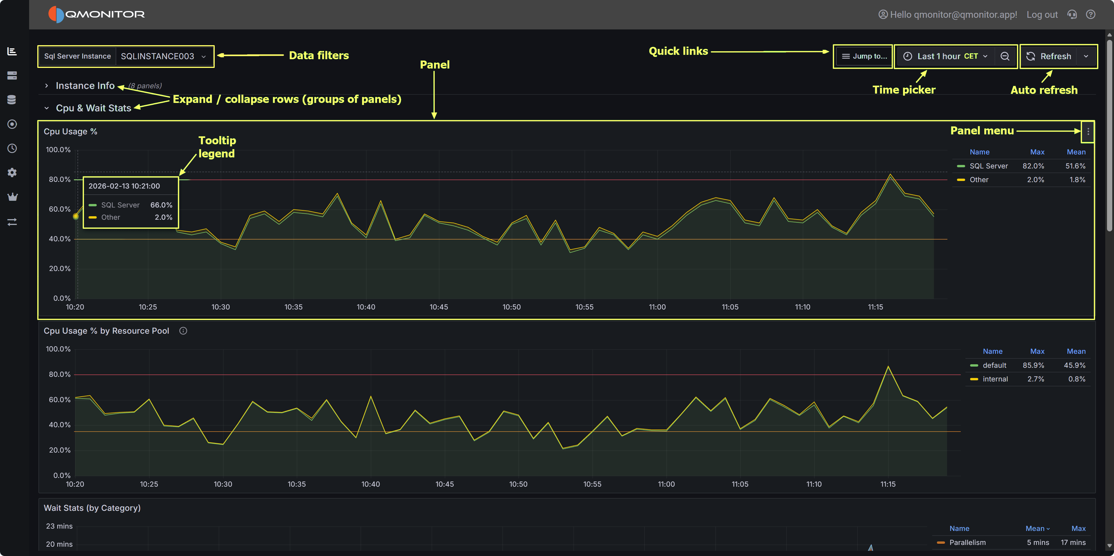QMonitor dashboard showing multiple metrics panels with time picker and filters

Time Range Selection

All the data in the dashboards can be filtered using the time picker on the top right corner: it offers predefined quick time ranges, like “Last 5 minutes”, “Last 1 hour”, “Last 7 days” and so on. These are usually the easiest way to select the time range.

If you want, you can also use absolute time ranges, that you can select with the calendar on the left side of the time picker popup. You can use the calendar buttons on the From and To fields to pick a date or you can enter the time range manually.

Panel Interactions

• Zoom: Click and drag on any graph to zoom into a specific time range
• Tooltips: Hover over data points to see exact values and timestamps
• Full Screen: Click the panel menu (⋮) and select “View” to expand a panel to full screen (press Escape to exit)
• Panel Menu: Click the three dots (⋮) in the top-right corner of any panel for additional options

Legend Controls

• Isolate a series: Click a legend item to show only that metric
• Toggle visibility: Ctrl+click to show/hide multiple series
• Sort: Some legends allow sorting by current value or name

Refresh and Auto-Update

• Use the refresh button (🔄) in the top-right to manually reload data
• Dashboards auto-refresh at intervals (typically every 30 seconds or 1 minute)
• The refresh interval is shown next to the refresh button

Instance and Database Filters

At the top of most dashboards, you’ll find dropdown filters to narrow your view:

• Instance: Select one or more SQL Server instances
• Database: Filter by specific databases (where applicable)
• Click “All” to select all options, or choose individual items

1.1 - Global Overview

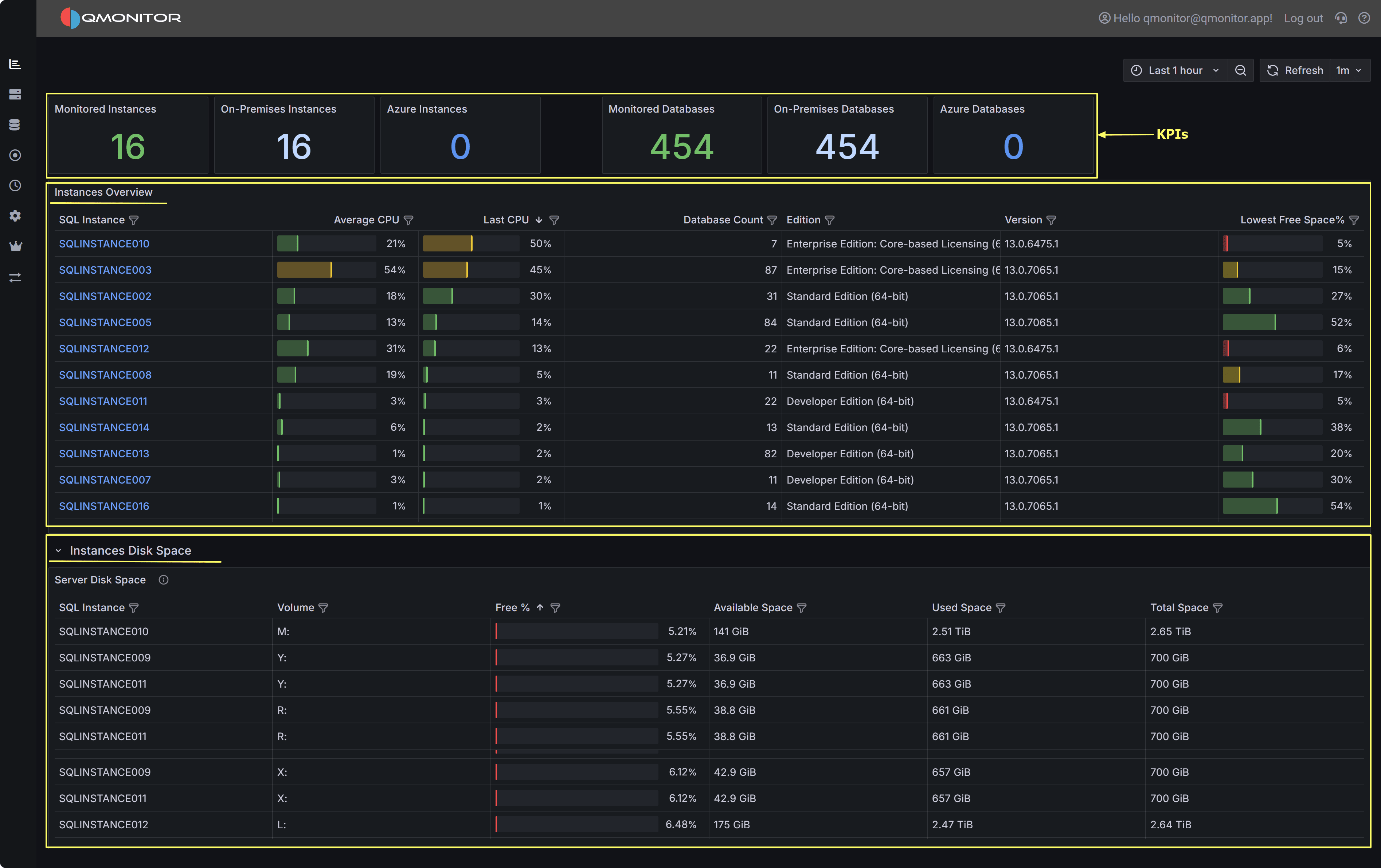
The Global Overview dashboard is your entry point to the SQL Server infrastructure: it provides an at-a-glance view of all the instances, along with useful performance metrics.

Global Overview dashboard showing instance KPIs, instances table, and disk space details

Dashboard Sections

Instance and Database Counts

At the top left of the dashboard, you have KPIs for the total number of monitored instances, divided between on-premises and Azure instances. At the top right you have the same KPI for the total number of monitored databases, again divided between on-premises and Azure.

Instances Overview

The middle of the dashboard contains the Instances Overview table, with the following information:

• SQL Instance: The name of the instance. For on-premises SQL Servers, this corresponds to the name returned by @@SERVERNAME, except that the backslash is replaced by a colon in named instances (you have SERVER:INSTANCE instead of SERVER\INSTANCE).
  For Azure SQL Managed Instances and Azure SQL Databases, the name is the network name of the logical instance. Click on the instance name to open the Instance Overview dashboard for that instance.
• Database: for Azure SQL Databases, the name of the database
• Elastic Pool: for Azure SQL Databases, the name of the elastic pool if in use, <No Pool> otherwise.
• Database Count: the number of databases in the instance
• Edition: the edition of SQL Server (Enterprise, Standard, Developer, Express). For Azure SQL Databases it is “Azure SQL Database”. For Azure SQL Managed Instances, it can be GeneralPurpose or BusinessCritical.
• Version: The version of SQL Server. For Azure SQL Database it contains the service tier (Basic, Standard, Premium…)
• Last CPU: the last value captured for CPU usage in the selected time interval
• Average CPU: the average CPU usage in the time interval
• Lowest disk space %: the percent of free space left in the disk that has the least space available. For Azure SQL Databases and Azure SQL Managed Instances the percentage is calculated on the maximum space available for the current tier.

Instances Disk Space

At the bottom of the dashboard, you have the detail of the disk space available on all instances. The table contains the following information:

• SQL Instance: the name of the instance, Azure SQL Database or Azure SQL Managed Instance.
• Database: for Azure SQL Databases, the name of the database
• Elastic Pool: for Azure SQL Databases, the name of the elastic pool if in use, <No Pool> otherwise.
• Volume: drive letter or mount point of the volume
• Free %: Percentage of free space in the volume
• Available Space: Available space in the volume. The unit measure is included in the value.
• Used Space: Used space in the volume
• Total Space: Size of the Volume (Used space + Available space)

1.2 - Instance Overview

This dashboard is one of the main sources of information to control the health and performance of a SQL Server instance. It contains the main performance metrics that describe the behavior of the instance over time.

Access this dashboard by clicking on an instance name from the Global Overview dashboard or by selecting it from the Instances dropdown at the top of any dashboard. Use the time picker to analyze historical performance or monitor real-time metrics. Each section can be expanded or collapsed to focus on specific areas of interest.

Dashboard Sections

The dashboard is divided into multiple sections, each one focused on a specific aspect of the instance performance.

Instance Info

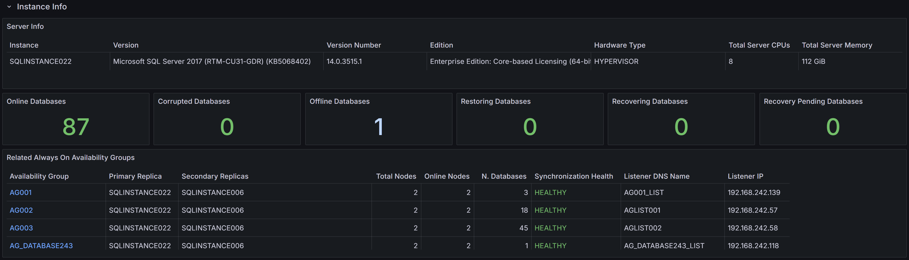Instance properties, database states, and Always On Availability Groups summary

At the top you can find the Instance Info section, where the properties of the instance are displayed. You have information about the name, version, edition of the instance, along with hardware resources available (Total Server CPUs and Total Server Memory).

You also have KPIs for the number of databases, with the counts for different states (online, corrupt, offline, restoring, recovering and recovery pending).

At the bottom of the section, you have a summary of the state of any configured Always On Availability Groups.

Cpu & Wait Stats

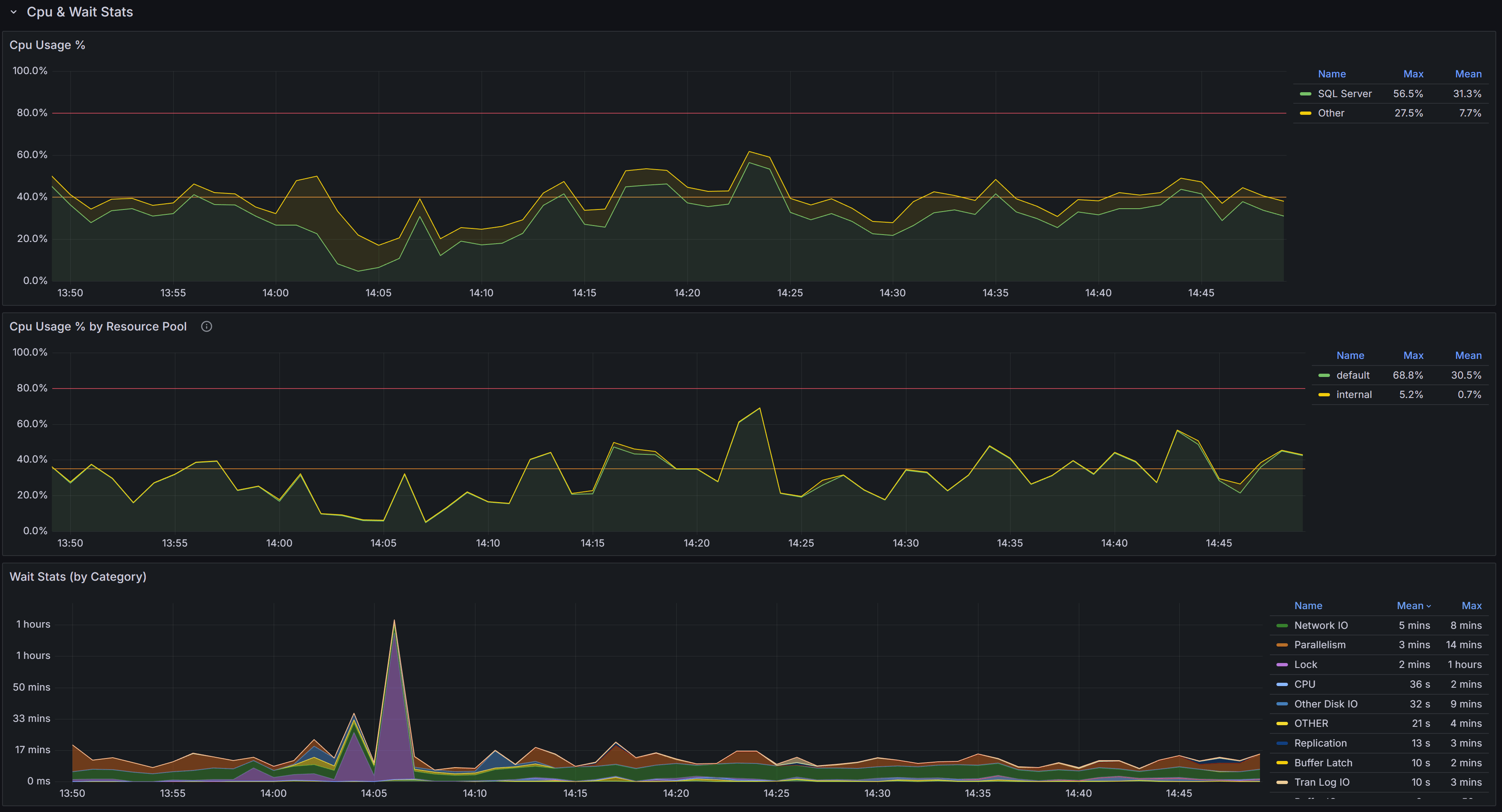Cpu, Cpu by Resource Pool and Wait Stats By Category

At the top of this section you have the chart that represents the percent CPU usage for the SQL Server process and for other processes on the same machine.

The second chart represents the percent CPU usage by resource pool. This chart will help you understand which parts of the workload are consuming the most CPU, according to the resource pool that you defined on the instance. If you are on an Azure SQL Managed Instance or on an Azure SQL Database, you will see the predefined resource pools available from Azure, while on an Enterprise or Developer edition you will see the user defined resource pools. For a Standard Edition, this chart will only show the internal pool.

The Wait Stats (by Category) chart represents the average wait time (per second) by wait category. The individual wait classes are not shown on this chart, which only represents wait categories: in order to inspect the wait classes, go to the Geek Stats dashboard.

Memory

Memory related metrics describe the state of the instance in respect to memory usage and memory pressure

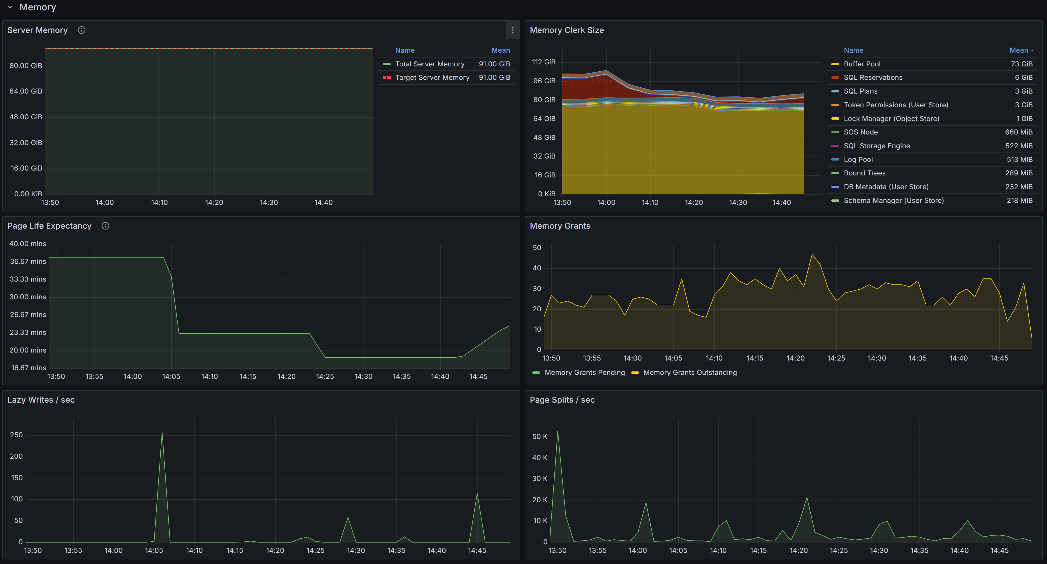
This section contains charts that display the state of the instance in respect to the use of memory. The chart at the top left is called “Server Memory”, and shows Target Server Memory vs Total Server Memory. The former represents the ideal amount of memory that the SQL Server process should be using, the latter is the amount of memory currently allocated to the SQL Server process. When the instance is under memory pressure, the target server memory is usually higher than total server memory.

The second chart shows the distribution of the memory between the memory clerks. A healthy SQL Server instance allocates most of the memory to the Buffer Pool memory clerk. Memory pressure could show on this chart as a fall in the amount of memory allocated to the Buffer Pool.
Another aspect to keep under control is the amount of memory used by the SQL Plans memory clerk. If SQL Server allocates too much memory to SQL Plans, it is possible that the cache is polluted by single-use ad-hoc plans.

The third chart displays Page Life Expectancy. This counter is defined as the amount of time that a database page is expected to live in the buffer cache before it is evicted to make room for other pages coming from disk. A very old recommendation from Microsoft was to keep this counter under 5 minutes every 4 Gb of RAM, but this threshold was identified in a time when most servers had mechanical disks and much less RAM than today.
Instead of focusing on a specific threshold, you should interpret this counter as the level of volatility of your buffer cache: a too low PLE may be accompanied by elevated disk activity and higher disk read latency.

Next to the PLE you have the Memory Grants chart, which represents the number of memory grant outstanding and pending. At any time, having Memory Grants Pending greater that zero is a strong indicator of memory pressure.

Lazy Writes / sec is a counter that represents the number of writes performed by the lazy writer process to eliminate dirty pages from the Buffer Pool outside of a checkpoint, in order to make room for other pages from disk. A very high number for this counter may indicate memory pressure.

Next you have the chart for Page Splits / sec, which represents how many page splits are happening on the instance every second. A page split happens every time there is not enough space in a page to accommodate new data and the original page has to be split in two pages.
Page splits are not desirable and have a negative impact on performance, especially because split pages are not completely full, so more pages are required to store the same amount of information in the Buffer Cache. This reduces the amount of data that can be cached, leading to more physical I/O operations.

Activity

General activity metrics, including user connections, compilations, transactions, and access methods

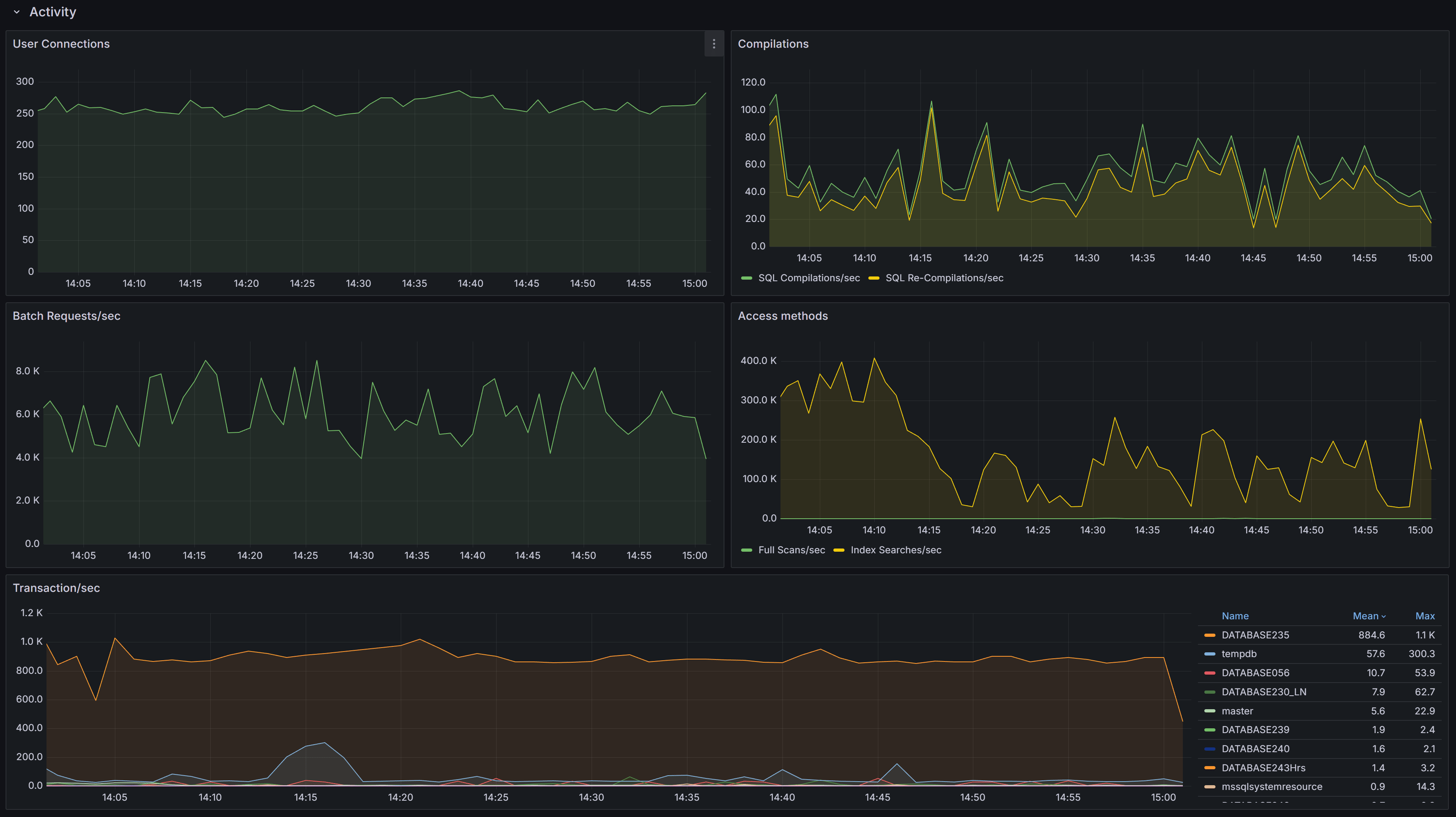
This section contains charts that display multiple SQL Server performance counters.

First you have the User Connections chart, which displays the number of active connections from user processes. This number should be consistent with then number of people or processes hitting the database and should not increase indefinitely (connection leak).

Next, we have the number of Compilations/sec vs Recompilations/sec. A healthy SQL Server database caches most of its execution plans for reuse, so that it does not need to compile a plan again: compiling plans is a CPU-intensive operation and SQL Server tries to avoid it as much as it can. A rule of thumb is to have a number of compilations per second that is 10% of the number of Batch Requests per second. A workload that contains a high number of ad-hoc queries will generate a higher rate of compilations per second.
Recompilations are very similar to compilations: SQL Server identifies in the cache a plan with one or more base objects that have changed and sends the plan to the optimizer to recompile it.
Compiles and recompiles are expensive operations and you should look for excessively high values for these counters if you suffer from CPU pressure on the instance.

The Access Methods chart displays Full Scans/sec vs Index Searches/sec. A typical OLTP system should get a low number of scans and a high number of Index Searches. On the other hand, a typical OLAP system will produce more scans.

The Transactions/sec panel displays the number of transactions/sec on the instance. This allows you to identify which database is under the higher load, compared to the ones that are not heavily utilized.

TempDB

Tempdb related metrics, including data and log space usage, active temp tables, and version store size

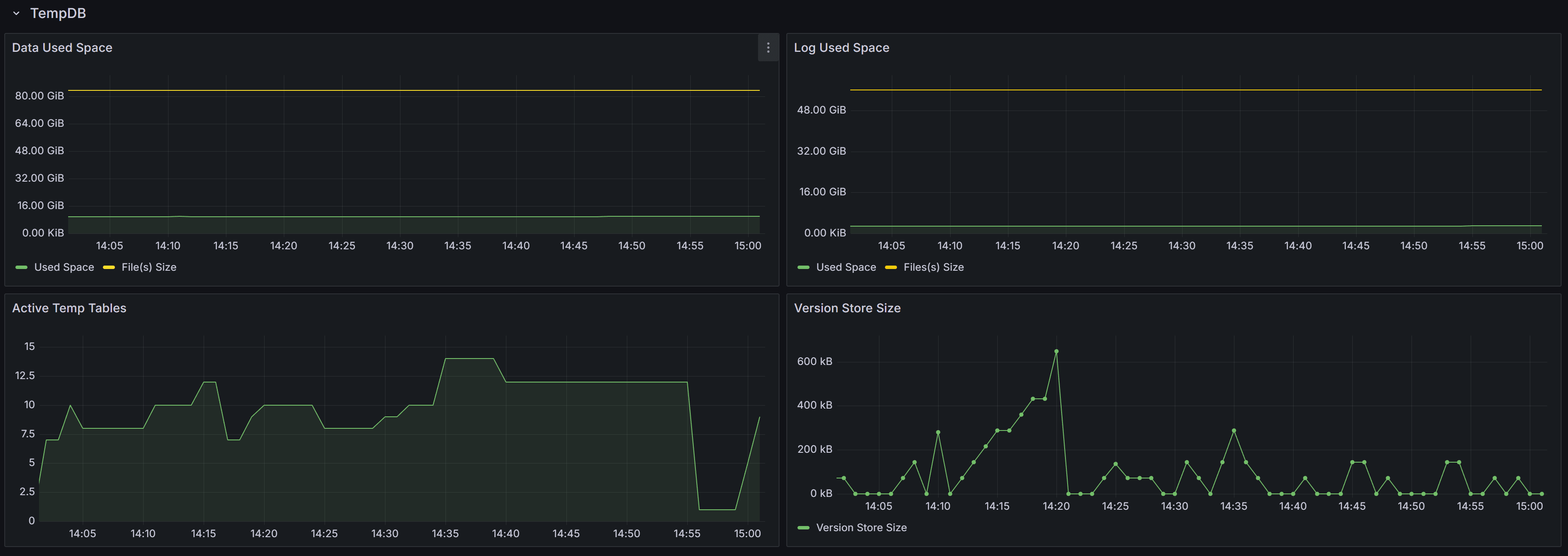
This section contains panels that describe the state of the Tempdb database. The tempdb database is a shared system database that is crucial for SQL Server performance.

The Data Used Space displays the allocated File(s) size compared to the actual Used Space in the database. Observing these metrics over time allows you to plan the size of your tempdb database, avoiding autogrow events. It also helps you size the database correctly, to avoid wasting too much disk space on a data file that is never entirely used by actual database pages.

The Log Used Space panel does the same, with log files.

Active Temp Tables shows the number of temporary tables in tempdb. This is not only the number of temporary tables created explicitly from the applications (table names with the # or ## prefix), but also worktables, spills, spools and other temporary objects used by SQL Server during the execution of queries.

The Version Store Size panel shows the size of the Version Store inside tempdb. The Version Store holds data for implementing optimistic locking by taking transaction-consistent snapshots of the data on the tables instead of imposing locks. If you see the size of Version Store going up continuously, you may have one or more open transactions that are not being committed or rolled back: in that case, look for long standing sessions with transaction count greater than one.

Database & Log Size

Size and growth of databases and transaction logs, with trends over time

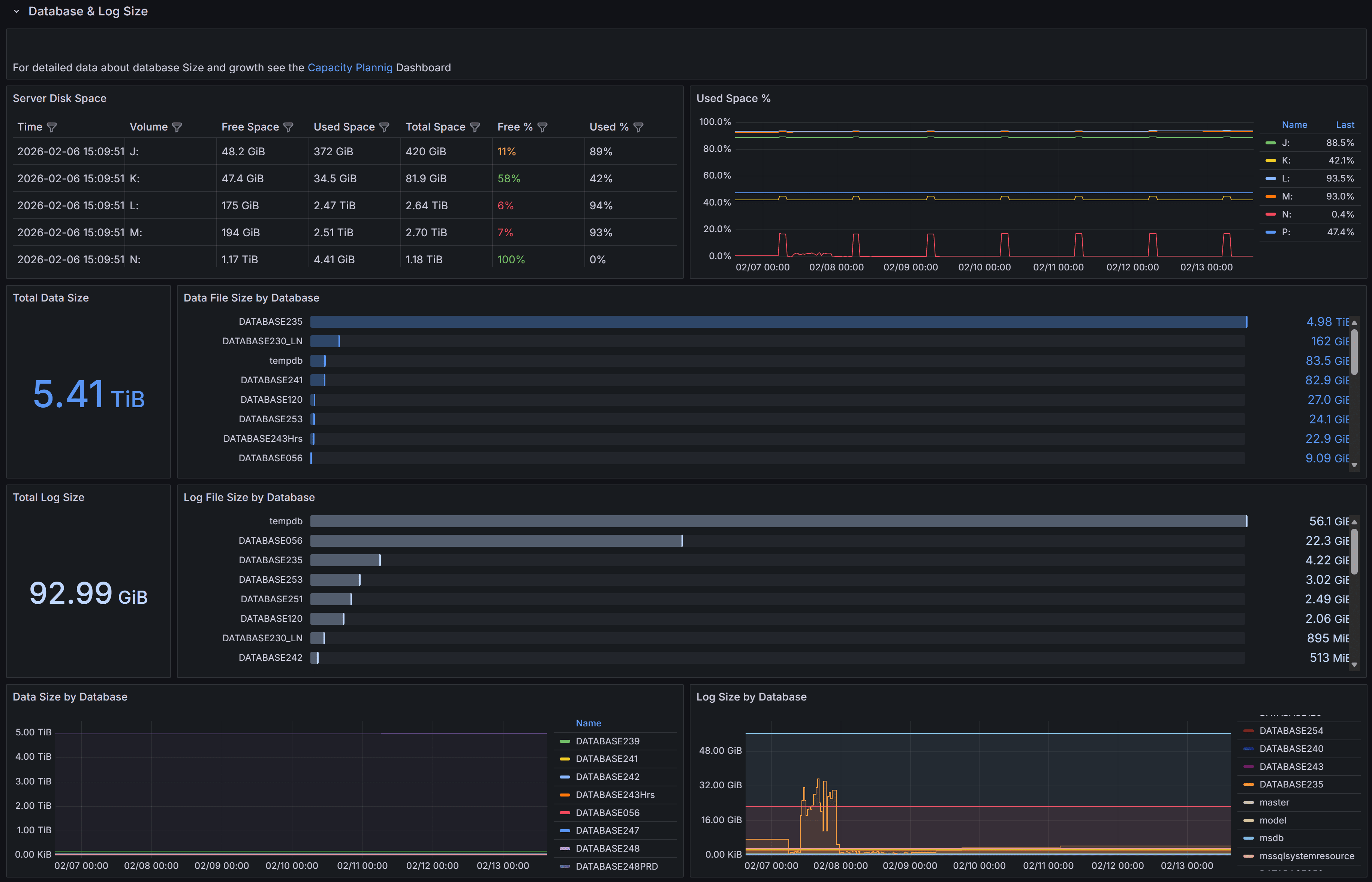
This section provides detailed information about the size and growth of databases and their transaction logs on the instance.

The Total Data Size panel displays the combined size of all data files across all databases on the instance. This metric helps you understand the overall storage footprint of your databases and plan for capacity requirements.

The Data File Size by Database chart shows a horizontal bar chart with the size of data files for each individual database. This visualization makes it easy to identify which databases consume the most storage space and helps prioritize storage optimization efforts.

The Total Log Size panel shows the cumulative size of all transaction log files on the instance. Monitoring log file size is important because transaction logs can grow rapidly under certain workloads, especially when full recovery mode is enabled and log backups are not performed frequently enough.

The Log File Size by Database chart presents the log file sizes for each database in a horizontal bar format. This allows you to quickly spot databases with unusually large transaction logs that may need attention, such as more frequent log backups or investigation of long-running transactions.

The Data Size by Database panel at the bottom left shows the size trend over time for each database. This time-series visualization helps you understand growth patterns and predict when additional storage capacity will be needed.

The Log Size by Database panel displays the transaction log size trend over time for each database. Sudden spikes in this chart may indicate unusual activity, such as large bulk operations, index maintenance, or uncommitted transactions that are preventing log truncation.

Database Volume I/O

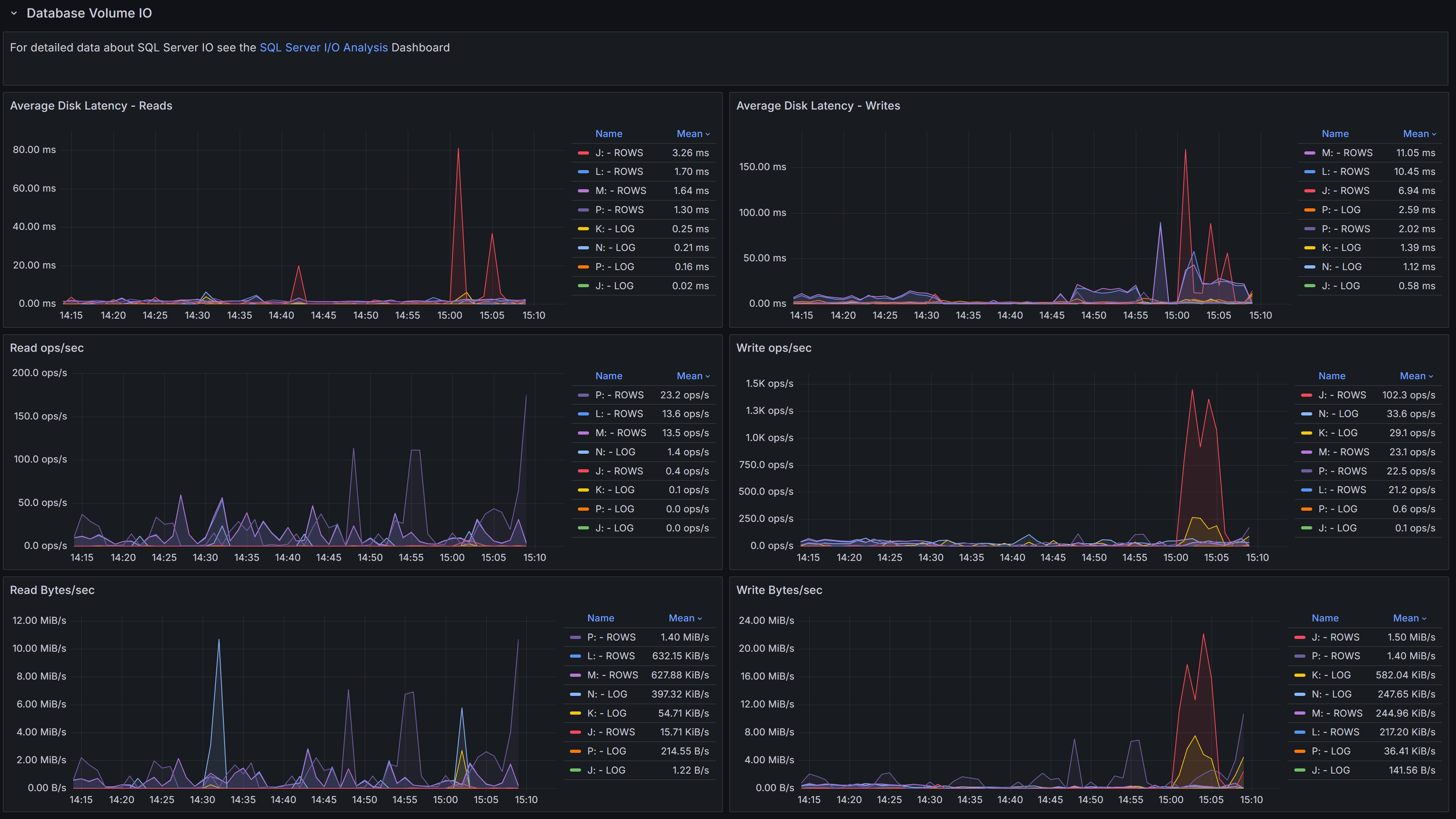Disk I/O performance metrics for volumes hosting database files, including latency, throughput, and operations per second

This section focuses on the I/O performance characteristics of the volumes hosting your databases. Understanding disk latency and throughput is essential for diagnosing performance problems related to storage.

The Average Data Latency - Reads chart displays the average read latency in milliseconds for data files. Read latency measures how long it takes for SQL Server to retrieve data from disk when it is not available in the buffer cache. For modern SSD storage, read latency should typically be under 5 milliseconds. Higher values may indicate storage performance issues, I/O contention, or inefficient queries causing excessive physical reads.

The Average Data Latency - Writes chart shows the average write latency in milliseconds for data files. Write operations occur when SQL Server flushes dirty pages from the buffer cache to disk during checkpoint operations or when the lazy writer needs to free up memory. Consistently high write latency can impact transaction commit times and overall system responsiveness.

The Read ops/sec panel displays the number of read operations per second on data files. This metric helps you understand the read workload intensity on your storage subsystem. A sudden increase in read operations may indicate missing indexes, insufficient memory causing more physical I/O, or changes in query patterns.

The Write ops/sec panel shows the number of write operations per second on data files. Write operations increase during periods of high transaction activity, bulk data loads, or index maintenance. Monitoring this metric helps you assess the write workload on your storage and identify periods of peak I/O activity.

The Read Bytes/sec chart represents the throughput in bytes per second for read operations. This metric, combined with read operations per second, gives you insight into the size of read I/O requests. Large sequential reads will show higher throughput with fewer operations, while random small reads will show more operations with lower throughput.

The Write Bytes/sec chart displays the throughput in bytes per second for write operations. This helps you understand the volume of data being written to disk over time. Monitoring write throughput is important for capacity planning and ensuring your storage subsystem can handle the write workload during peak periods.

Queries

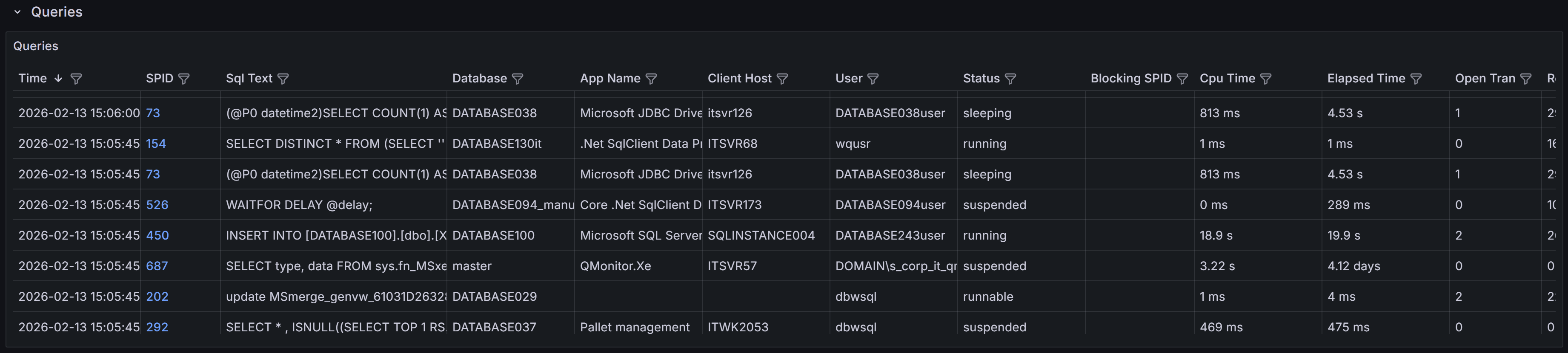Queries captured, with details on execution, resource usage, and wait information for troubleshooting performance issues

This section provides visibility into the queries running on the instance. The Queries table at the bottom of the dashboard lists all queries captured during the selected time range. A capture is performed every 15 seconds, and the table is updated in real time as new queries are captured, according to the refresh interval defined for the dashboard. This table is a powerful tool for identifying and investigating problematic queries that may be impacting the performance of your SQL Server instance. It is also a great way to troubleshoot performance issues in real time or in the past, by selecting a specific time range.

The table includes the following columns to help you identify and investigate problematic queries:

• Time shows the timestamp when the query was captured.
• SPID (Server Process ID) identifies the session that is executing the query. Click on the SPID to show more details about the query in the query detail dashboard.
• Sql Text presents a snippet of the query text, truncated to 255 characters. Click on the SPID to see the full statement.
• Database identifies which database the query is running against.
• App Name shows the application name that is connected to the instance and running the query. This information is provided by the client application when it connects to SQL Server.
• Client Host reveals which machine is executing the query.
• User displays the SQL Server login name used to run the query.
• Status indicates whether the query is currently running, suspended, or completed.
• Blocking SPID shows if the query is blocked by another session, with the session ID of the blocking process.
• Cpu Time displays the cumulative CPU time consumed by the query in milliseconds.
• Elapsed Time shows the total wall-clock time the query has been running.
• Open Tran indicates the number of open transactions for the session, which is important for identifying long-running transactions that may cause blocking or prevent log truncation.
• Reads shows the number of logical reads performed by the query, which is a key indicator of query efficiency and resource consumption.
• Writes displays the number of logical writes performed by the query. High write counts may indicate operations that modify large amounts of data or queries that create temporary objects or worktables.
• Query Hash is a binary hash value that identifies queries with similar logic, even if literal values differ. This allows you to group and analyze similar queries together to identify patterns in query execution. Click on the hash value to see all queries with the same query hash in the query detail dashboard.
• Plan Hash is a binary hash value that identifies queries using the same execution plan. Multiple queries with the same plan hash share the same plan in the cache, which helps you understand plan reuse and cache efficiency. Click on the hash value to download the execution plan for the query in XML format.
• Wait Type shows the type of wait the session is currently experiencing if it is in a suspended state. Common wait types include PAGEIOLATCH for disk I/O, CXPACKET for parallelism coordination, and LCK for lock waits. Understanding wait types helps diagnose the root cause of query delays.
• Wait Resource displays the specific resource the session is waiting for, such as a page ID, lock resource, or network address. This information is valuable for pinpointing exactly what is causing a query to wait.
• Time since last request shows how long the session has been idle since its last batch completed. Sessions with long idle times but open transactions may be holding locks unnecessarily and causing blocking issues.
• Blocking or blocked displays whether the session is blocking other queries, being blocked, or both. This helps you quickly identify sessions involved in blocking chains and prioritize resolution efforts.

Each table column allows you to sort and filter the queries to focus on specific criteria, such as high CPU time, long elapsed time, or specific wait types. You can also use the filter on the time column to focus on queries captured at a specific time, such as the latest available sample.

The column filters work more or less like Excel filters: you can select specific values to include or exclude, or you can use the search box to find specific text in the column.

Use this table to identify queries that may need optimization, such as those with high CPU time, excessive reads, or long elapsed times. Queries that are frequently blocked or have open transactions for extended periods may indicate locking or transaction management issues that require investigation. Click on any SPID to drill down into more details and view the full query text and execution plan when available.

1.2.1 - Query Detail

The Query Detail dashboard displays details for a single SQL query.

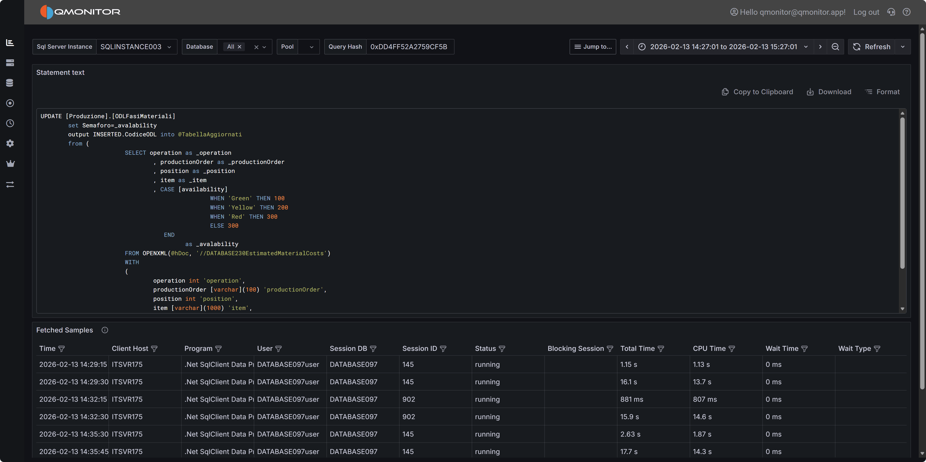Query Detail Dashboard

Dashboard Sections

Query Text and Actions

The top panel shows the query text as QMonitor captured it. Queries generated by ORMs or written on a single line can be hard to read. Click “Format” to apply readable SQL formatting.

Click “Copy to Clipboard” to copy the query for running or analysis in external tools (such as SSMS). Use “Download” to save the query as a .sql file.

Fetched Samples

The table below lists all executions of this query within the selected time range. QMonitor captures a sample every 15 seconds: long-running queries will produce multiple samples, and queries running at the instant of capture will produce a sample as well.

Samples alone may not fully reflect a query’s resource usage or execution time. For a complete impact analysis, rely on the Query Stats data: Query Stats.

1.3 - Query Stats

The Query Stats dashboard summarizes workload characteristics and surfaces high cost queries so you can prioritize tuning and capacity decisions. This dashboard is your primary tool for understanding which queries consume the most resources and where optimization efforts will have the greatest impact.

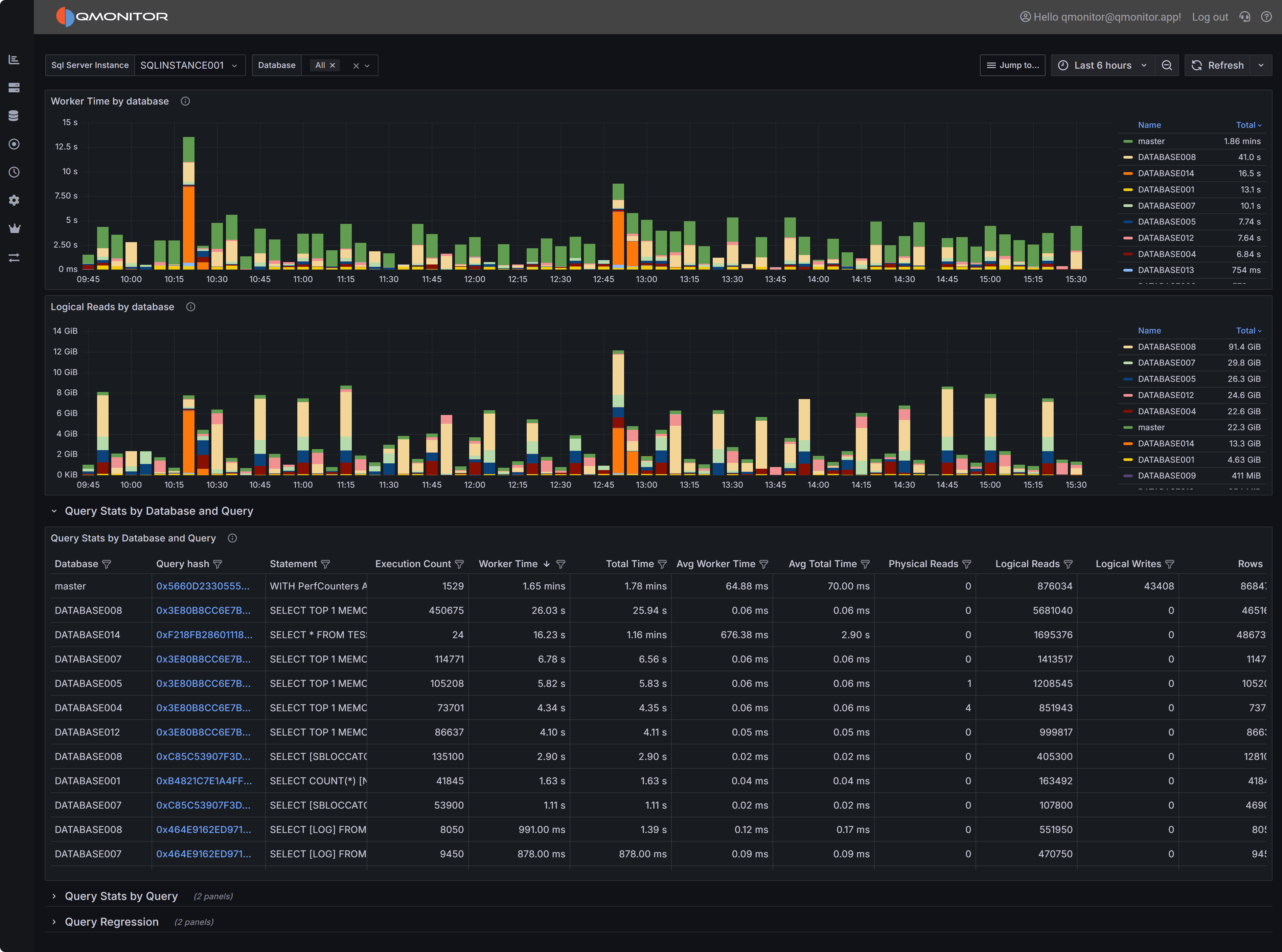Query Stats Dashboard showing workload overview and query statistics

Dashboard Sections

Workload Overview

At the top of the dashboard you have two charts that provide a high-level view of resource consumption across your databases.

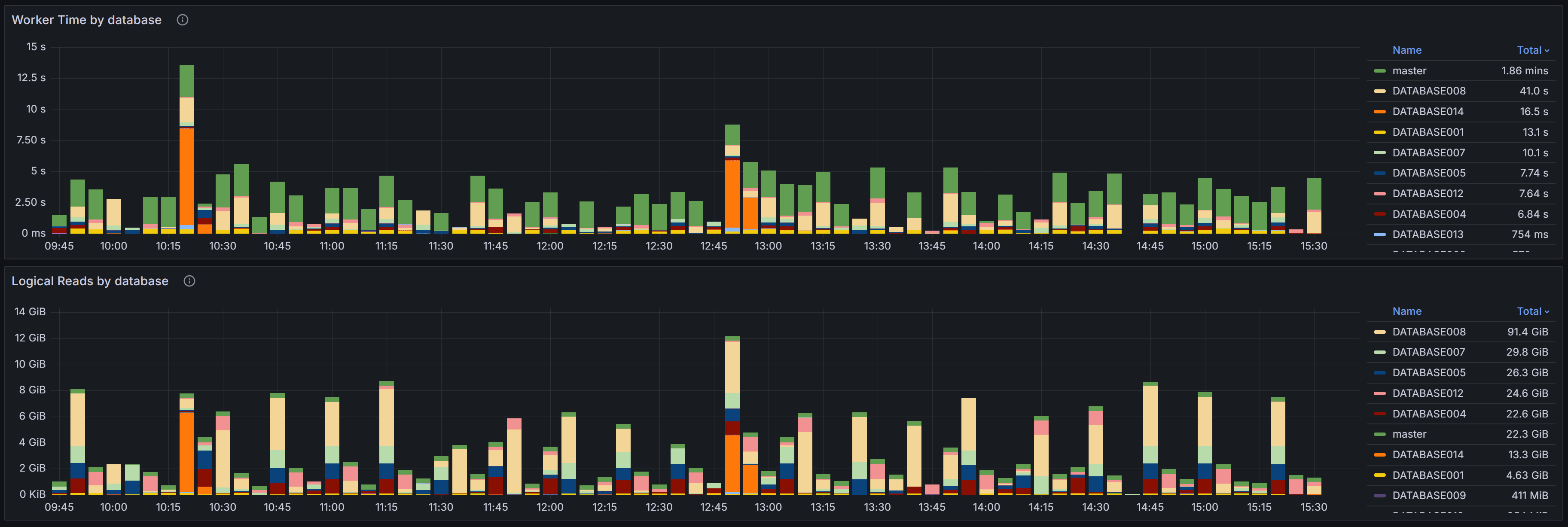Query Stats Overview

The Worker Time by Database chart shows the cumulative CPU time consumed by queries in each database during the selected time range. Worker time represents the actual CPU cycles spent executing queries, making it one of the most important metrics for understanding which databases are driving CPU usage on your instance. By analyzing this chart over time, you can identify databases that consistently consume high CPU resources or spot sudden increases that may indicate new workloads or inefficient queries. This information is valuable when planning capacity, troubleshooting performance issues, or identifying which databases deserve the most tuning attention.

The Logical Reads by Database chart displays the number of logical page reads performed by queries in each database. Logical reads measure how many 8KB pages SQL Server accessed from memory or disk to satisfy query requests. High logical reads indicate either large result sets, missing indexes forcing table scans, or inefficient query patterns that read more data than necessary. Unlike physical reads which measure actual disk I/O, logical reads capture all data access regardless of whether the page was in cache or required a disk read. Databases with high or rising logical reads may suffer from I/O pressure, especially if memory is limited and pages must be read from disk frequently. Use this chart to compare databases and track whether optimization efforts are reducing unnecessary data access.

Query Stats by Database and Query

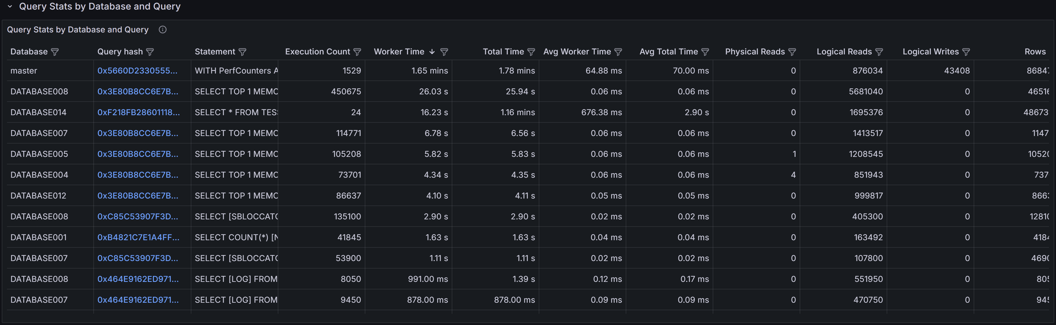Query Stats By Database and Query

This section shows the top queries grouped by both database and query text. Each row in the table represents a specific query running in a specific database, allowing you to drill down into the most resource-intensive queries within individual databases.

The table includes several key metrics to help you assess query performance. Worker Time displays the cumulative CPU time consumed by all executions of this query. Logical Reads shows the total number of pages read from the buffer pool across all executions. Duration represents the total elapsed wall-clock time for all executions, which may be higher than worker time when queries wait for resources like locks or I/O. Execution Count tells you how many times the query has run during the selected time period.

Understanding the relationship between these metrics is crucial for effective tuning. A query with high cumulative worker time and many executions might benefit from better indexing to reduce the cost per execution. A query with high worker time but few executions may have an inefficient execution plan that needs rewriting or better statistics. High duration relative to worker time suggests the query spends significant time waiting rather than executing, pointing to blocking, I/O latency, or resource contention issues.

Use the filters at the top of the table to narrow your analysis by database name, application name, or client host. This helps you focus on specific workloads or troubleshoot issues reported by particular applications. Sort the table by different columns to identify queries with the highest cumulative cost, longest individual executions, or most frequent execution patterns. Click any row to open the query detail dashboard where you can examine the full query text, execution plans, and detailed runtime statistics.

Query Stats by Query

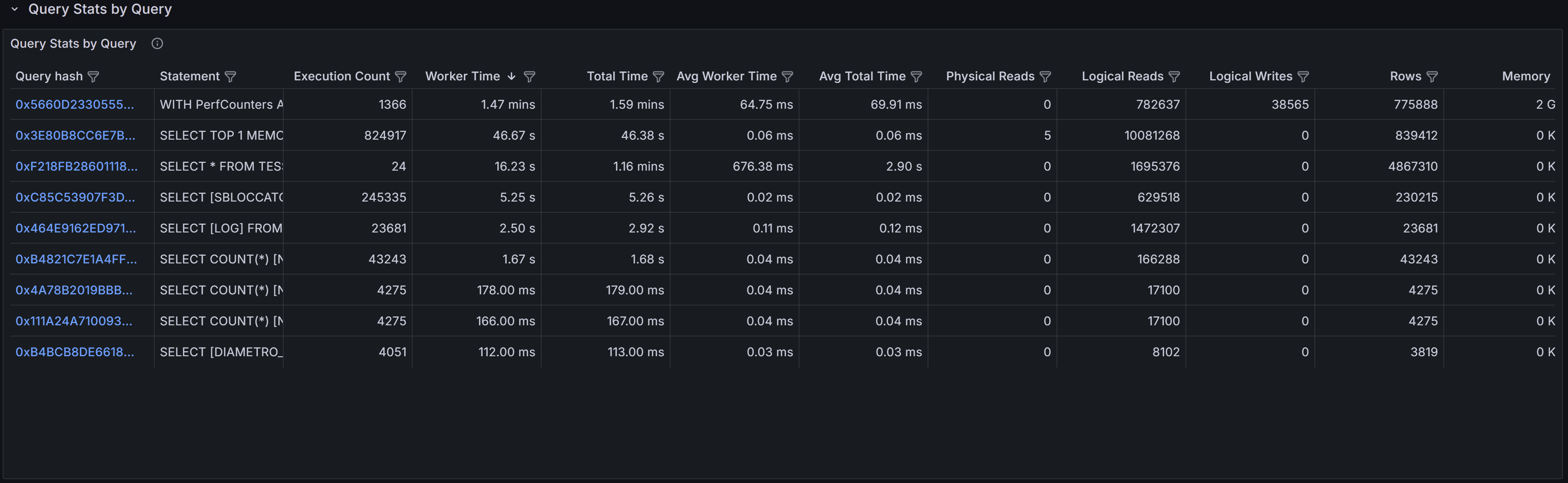Query Stats By Query

The Query Stats by Query section aggregates statistics across all databases for queries with identical or similar text. This view is particularly useful for identifying widely-used queries that appear in multiple databases, a common pattern in multi-tenant applications where the same queries run against different tenant databases.

By aggregating across databases, you can see the total impact of a specific query pattern on your entire instance. A query that seems moderately expensive in a single database might actually be consuming significant resources when its cumulative cost across dozens of tenant databases is considered. This view helps you prioritize optimization efforts toward queries that will have the broadest impact across your infrastructure.

The columns in this table provide both cumulative totals and per-execution averages. Total Worker Time and Total Logical Reads show the combined cost across all databases and executions, while Average Worker Time and Average Logical Reads indicate the typical cost of a single execution. High averages suggest inefficient query plans that need tuning, while high totals with low averages indicate frequently-executed queries that might benefit from caching, result set optimization, or better application-level batching.

This section is especially valuable for detecting candidates for query parameterization. If you see similar query text with slightly different literal values appearing as separate entries, these queries may not be using parameterized queries or prepared statements, leading to plan cache pollution and increased compilation overhead. Converting these to parameterized queries can reduce CPU usage and improve plan reuse.

Query Regressions

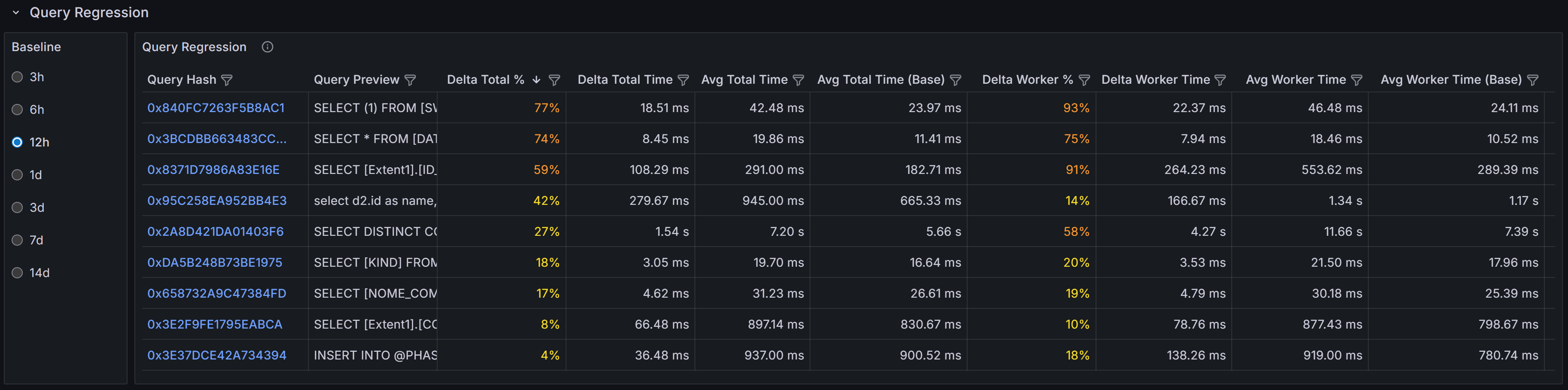Query Regressions

The Query Regressions section highlights queries whose performance has degraded significantly compared to their historical baseline. Performance regressions often occur after SQL Server chooses a different execution plan due to statistics updates, parameter sniffing issues, schema changes, or increases in data volume.

This section compares query performance during the selected time window against previous periods to identify substantial increases in duration, CPU consumption, or logical reads. Regressions are typically caused by execution plan changes, shifts in data distribution that make existing plans inefficient, increased blocking as concurrency grows, or resource contention from other workloads. When a query suddenly takes longer to execute or consumes more CPU than it did previously, investigating the execution plan history can reveal whether SQL Server switched from an efficient index seek to a costly table scan, or from a nested loop join to a less optimal hash join.

Click on a query hash value to drill into the detailed execution history for that query. The query detail view shows historical execution plans, runtime statistics over time, and the complete query text. By comparing current and historical plans side by side, you can identify exactly what changed and decide whether to force a specific plan, update statistics, add missing indexes, or rewrite the query to avoid plan instability.

Query regressions are particularly important to monitor because they represent sudden performance changes that may not be caused by code changes. A query that worked well for months can suddenly become a performance problem without any application deployment, making these issues challenging to diagnose without historical performance data.

Data Sources and Query Store Integration

Query statistics displayed in this dashboard are gathered from two primary sources depending on your SQL Server configuration and version.

QMonitor continuously captures query execution data through snapshots of the query stats DMVs, providing query statistics even when Query Store is not available or disabled. This capture gives you visibility into query performance across all SQL Server versions and editions that QMonitor supports.

When Query Store is enabled on your databases, QMonitor integrates Query Store data into the dashboard to provide richer historical information. Query Store is a SQL Server feature introduced in SQL Server 2016 that automatically captures query execution plans, runtime statistics, and performance metrics. It is enabled at the database level and retains historical data of query executions, even for queries that are no longer in the plan cache or are never available in the cache.

Qmonitor tries to rely on query store data when available, but if query store is disabled or not supported on your SQL Server version, it will fall back to using the query stats DMVs for real-time data. While you will still see query performance data, you may have less historical plan information and fewer options for plan comparison. Enabling Query Store on your production databases is recommended for comprehensive query performance monitoring and troubleshooting.

1.3.1 - Query Stats Detail

The Query Stats Detail dashboard focuses on a single query and shows how each compiled plan for that query performed over the selected time interval. This dashboard is your primary tool for understanding query performance variations, comparing execution plans, and diagnosing performance issues at the individual query level.

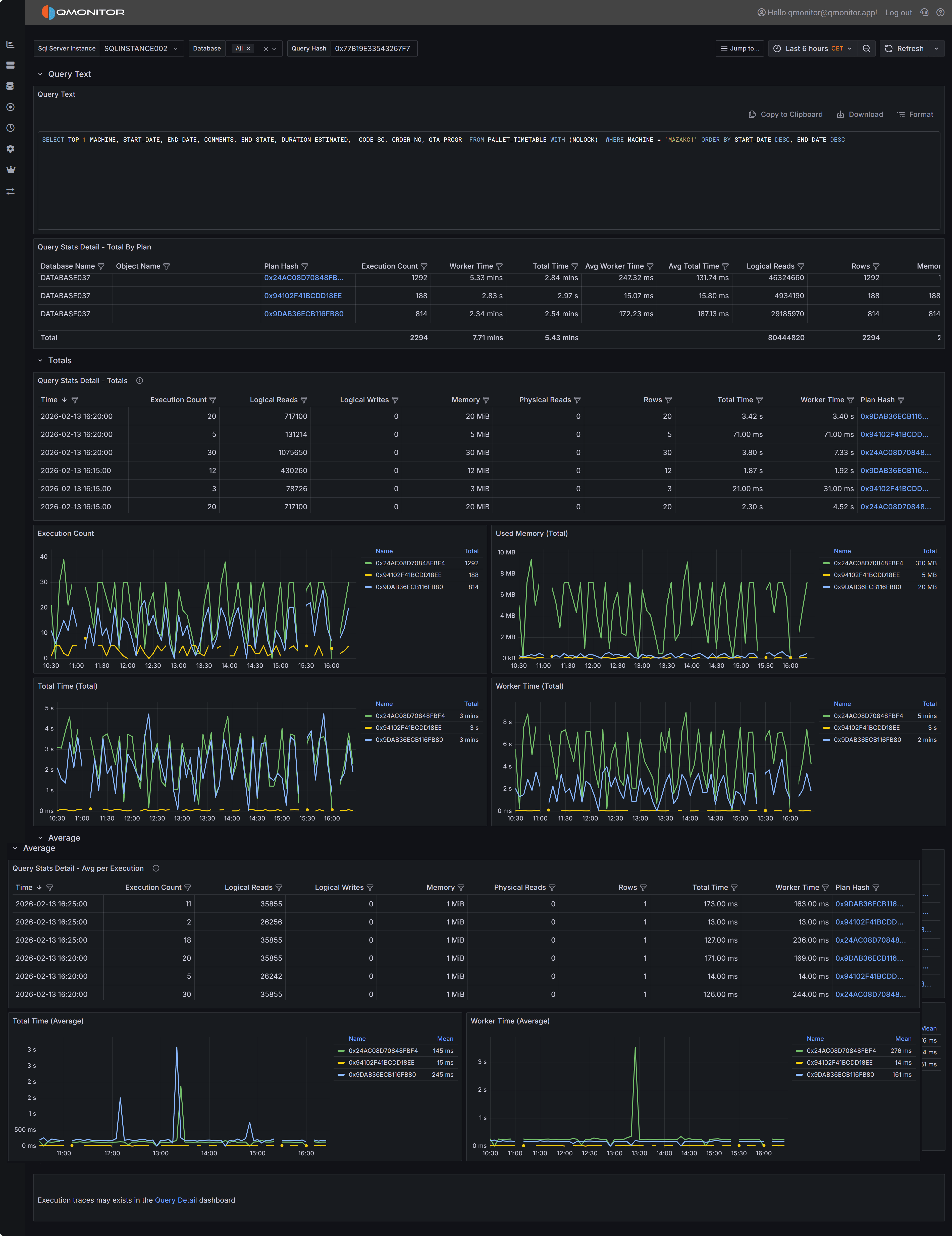Query Stats Detail dashboard showing query text, plan summaries, and performance metrics

Dashboard Sections

Query Text Display

At the top of the dashboard you will find the complete SQL text for the query you are investigating.

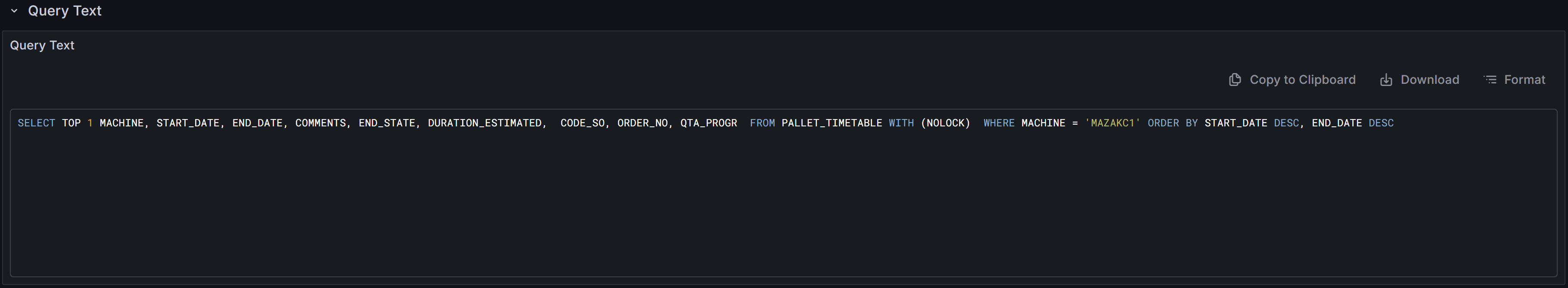Query text display with copy, download, and format controls

The toolbar above the query text provides several useful functions. The copy button allows you to quickly copy the entire query text to your clipboard so you can paste it into SQL Server Management Studio or another query editor for testing and optimization. The download button saves the query text as a SQL file to your local machine, which is useful when you need to share the query with colleagues or save it for documentation purposes. The format button reformats the query text with proper indentation and line breaks, making complex queries easier to read and understand. Properly formatted queries are particularly helpful when analyzing deeply nested subqueries or queries with many joins and predicates.

Plans Summary Table (Totals by Plan)

The Plans Summary table provides a high-level comparison of all execution plans that SQL Server has compiled for this query during the selected time range. Each row in the table represents a distinct execution plan, identified by its plan hash value.

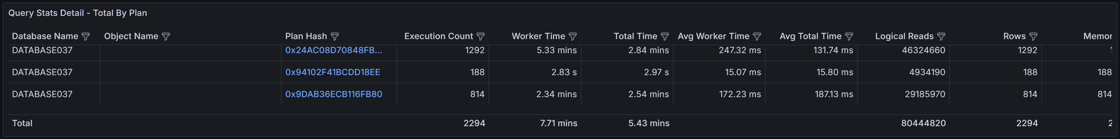Plans summary showing execution counts and performance metrics for each plan

The table includes several key metrics to help you compare plan performance.

• Database Name indicates which database the query ran in
• Object Name shows the name of the stored procedure, function, or view that contains the query, if applicable.
• Execution Count shows how many times each plan was executed during the time range.
• Worker Time displays the total CPU time consumed by all executions of this plan.
• Total Time represents the total elapsed wall-clock time, which includes both execution time and any waiting time for resources.
• Average Worker Time and Average Total Time show the per-execution cost, helping you identify plans that are individually expensive versus plans that accumulate high cost through frequent execution.
• Rows indicates the number of rows returned by the query, which can help you identify whether different plans are returning different result sets or processing different amounts of data.
• Memory Grant shows the total memory allocated to executions of this plan.

This table is particularly valuable for identifying plan variations and understanding their performance impact. If you see multiple plans with significantly different performance characteristics for the same query text, this often indicates parameter sniffing issues where SQL Server cached different plans optimized for different parameter values. Plans with high average worker time or total time deserve investigation to understand what makes them expensive. Plans with very high execution counts but low average cost might benefit from application-level caching or query result reuse rather than query-level optimization.

Totals Section

The Totals section displays time-series data showing how query performance varied over the selected time range. The data is aggregated into 5-minute buckets, with each row representing the cumulative metrics for all query executions that occurred during that 5-minute period.

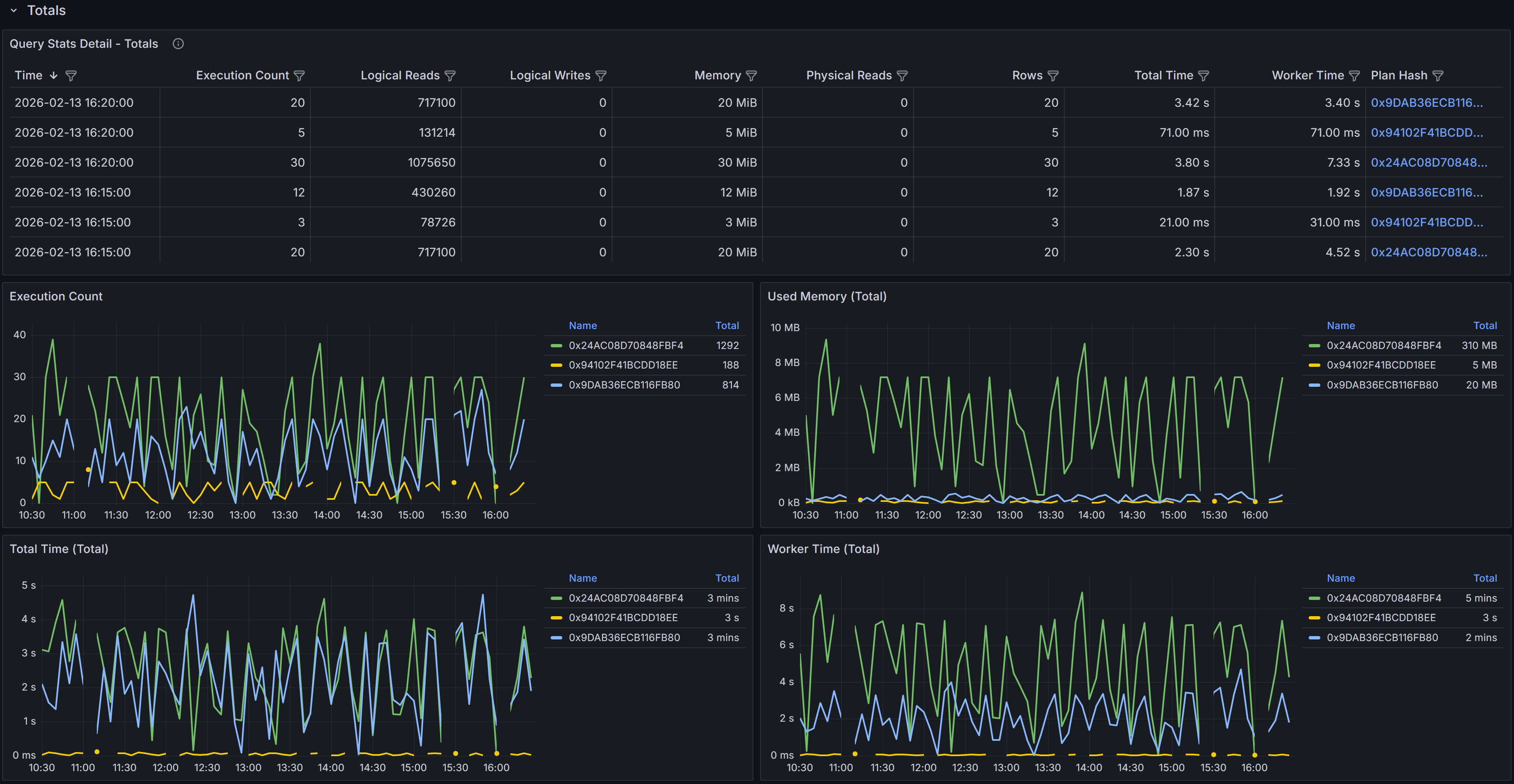Time-series table and charts showing cumulative query performance metrics

The time-series table includes detailed metrics for each 5-minute bucket.

• Time shows when the 5-minute bucket started.
• Execution Count indicates how many times the query ran during that period.
• Logical Reads displays the total number of 8KB pages read from memory during all executions in the bucket.
• Logical Writes shows the total pages written.
• Memory represents the cumulative memory grants for all executions.
• Physical Reads indicates how many pages had to be read from disk because they were not in the buffer cache.
• Rows shows the total number of rows returned by all executions.
• Total Time represents the cumulative elapsed time for all executions
• Worker Time shows the cumulative CPU time.
• Plan Hash identifies which plan was used during each sample period.

The Plan Hash values in the table are clickable links. When you click a plan hash, QMonitor downloads the execution plan as a .sqlplan file that you can open in SQL Server Management Studio.

The charts in the Totals section visualize how query performance varied over time and how different plans contributed to resource consumption. The Execution Count by Plan chart shows how frequently each plan was executed during each time bucket, helping you understand plan usage patterns. The Memory by Plan chart displays memory grant trends, which is valuable for identifying queries that request excessive memory or queries whose memory requirements vary significantly over time. The Total Time by Plan and Worker Time by Plan charts show how much elapsed time and CPU time each plan consumed, making it easy to spot periods when query performance degraded or when a particular plan dominated resource usage.

Averages Section

The Averages section presents the same time-series data as the Totals section, but with metrics averaged per execution rather than aggregated cumulatively. This view is particularly valuable for understanding the per-execution cost of the query and identifying when individual executions became more expensive.

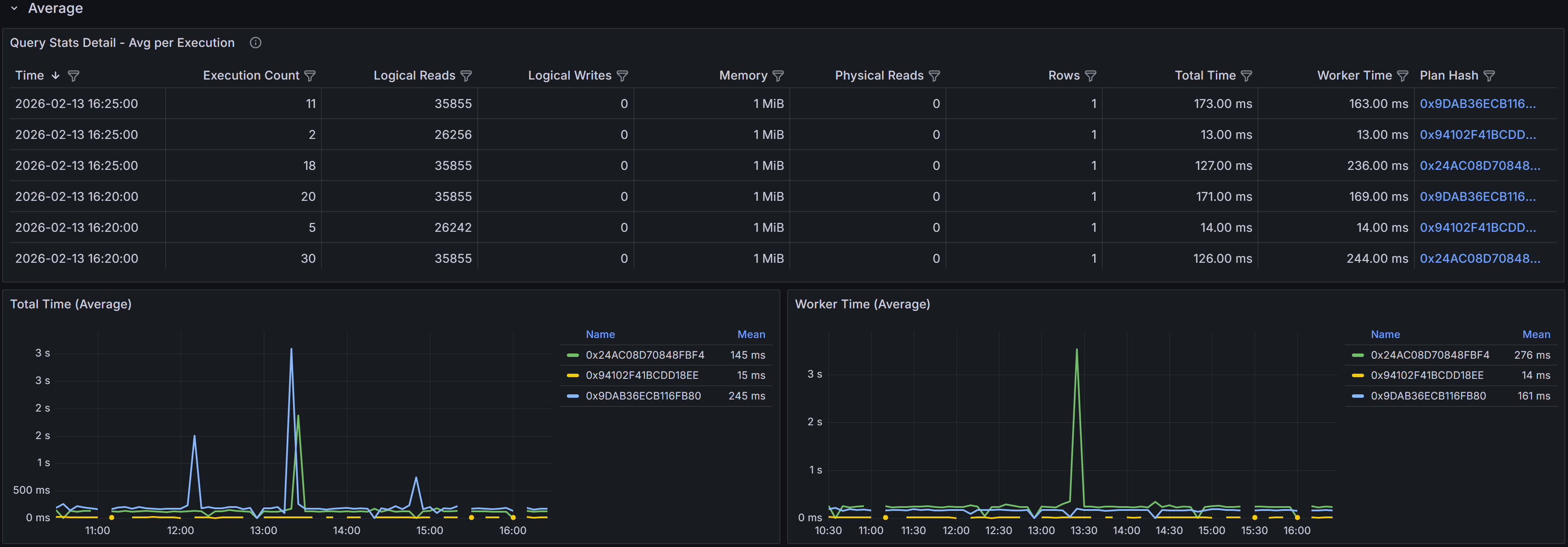Time-series table and charts showing average per-execution metrics

The time-series table in the Averages section shows metrics averaged across all executions that occurred during each 5-minute bucket. For example, if the query executed 100 times during a 5-minute period with a total worker time of 50,000 milliseconds, the average worker time would be 500 milliseconds per execution. This per-execution perspective helps you identify whether query performance degradation is due to the query becoming inherently more expensive or simply running more frequently.

The columns mirror those in the Totals table: Sample Time, Execution Count, averaged Logical Reads, Logical Writes, Memory, Physical Reads, Rows, Total Time, Worker Time, and Plan Hash. The Execution Count is not averaged since it represents the number of times the query ran, but all other metrics show the average value per execution during that time bucket.

The charts in the Averages section focus on per-execution cost trends. The Total Time (avg) by Plan chart shows how the average elapsed time per execution varied over time for each plan. The Worker Time (avg) by Plan chart displays the average CPU time per execution. These charts help you distinguish between performance issues caused by increased query frequency versus issues caused by increased per-execution cost.

Investigating Query Performance

When analyzing query performance using this dashboard, start by examining the Plans Summary table to understand how many distinct plans exist for the query and whether any plans are significantly more expensive than others. Multiple plans with different performance characteristics often indicate parameter sniffing issues where SQL Server cached plans optimized for specific parameter values that may not be optimal for all parameter combinations.

Use the Totals and Averages charts together to understand performance patterns. High totals with low averages suggest the query runs frequently but each execution is relatively cheap, pointing to application-level optimization opportunities. High averages indicate expensive individual executions that need query-level optimization. Comparing performance across different time periods helps you identify whether performance degradation was gradual or sudden, which provides clues about the root cause.

Using the Dashboard Effectively

Set the time range selector to focus on the period when performance issues occurred. If you are investigating a regression that started yesterday, select a time range that includes both before and after the regression so you can compare plan behavior and metrics. For ongoing performance issues, use a recent time range like the last few hours to analyze current behavior.

Sort and filter the time-series tables to focus on specific time periods or plans. If you know that performance degraded at a specific time, filter the table to show only samples from that period. If you want to compare two different plans, filter by plan hash to isolate their metrics.

Download multiple execution plans when comparing plan variations. Open them side by side in SQL Server Management Studio to identify exactly what changed between plans. Look for differences in join types, index selection, join order, and operator choices. Understanding why SQL Server chose different plans helps you decide whether to update statistics, add indexes, use query hints, or enable plan forcing.

When you identify a specific plan that performs best, consider using Query Store plan forcing to lock the query to that plan. This prevents SQL Server from choosing suboptimal plans in the future, providing stable and predictable performance. However, plan forcing should be used carefully and monitored regularly, as data volume changes or schema changes may eventually make the forced plan suboptimal.

Compare Totals and Averages to determine whether optimization efforts should focus on reducing per-execution cost or reducing execution frequency. If totals are high but averages are low, work with application teams to reduce unnecessary query executions, implement caching, or batch operations. If averages are high, focus on database-level optimization like indexes, query rewrites, or schema changes.

1.4 - SQL Server Events

The Events dashboard shows the number of events that occurred on the SQL Server instance during the selected time range.

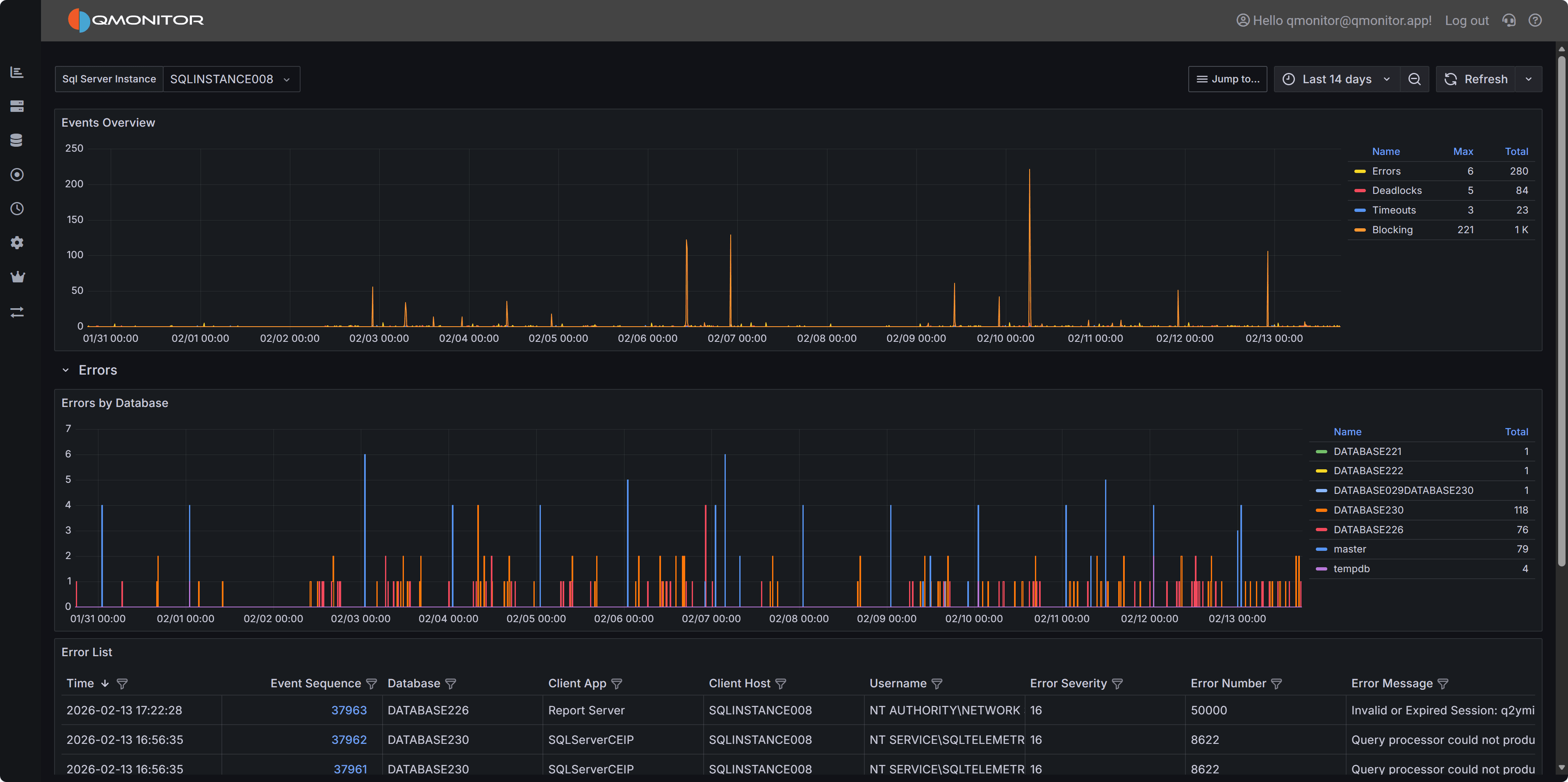SQL Server Events dashboard showing events by type

The top chart breaks events down by type:

• Errors
• Deadlocks
• Blocking
• Timeouts

Expand a row to view a chart for that event type by database and a list of individual events. Click a row’s hyperlink to open a detailed dashboard for that event type, where you can inspect the event details.

1.4.1 - Errors

The Errors dashboard helps you monitor and diagnose SQL Server errors that may indicate application issues, security problems, or infrastructure failures. By tracking error patterns over time and analyzing error details, you can proactively identify and resolve problems before they impact users.

Expand the “Errors” row to see a chart that shows the number of errors per database over time.

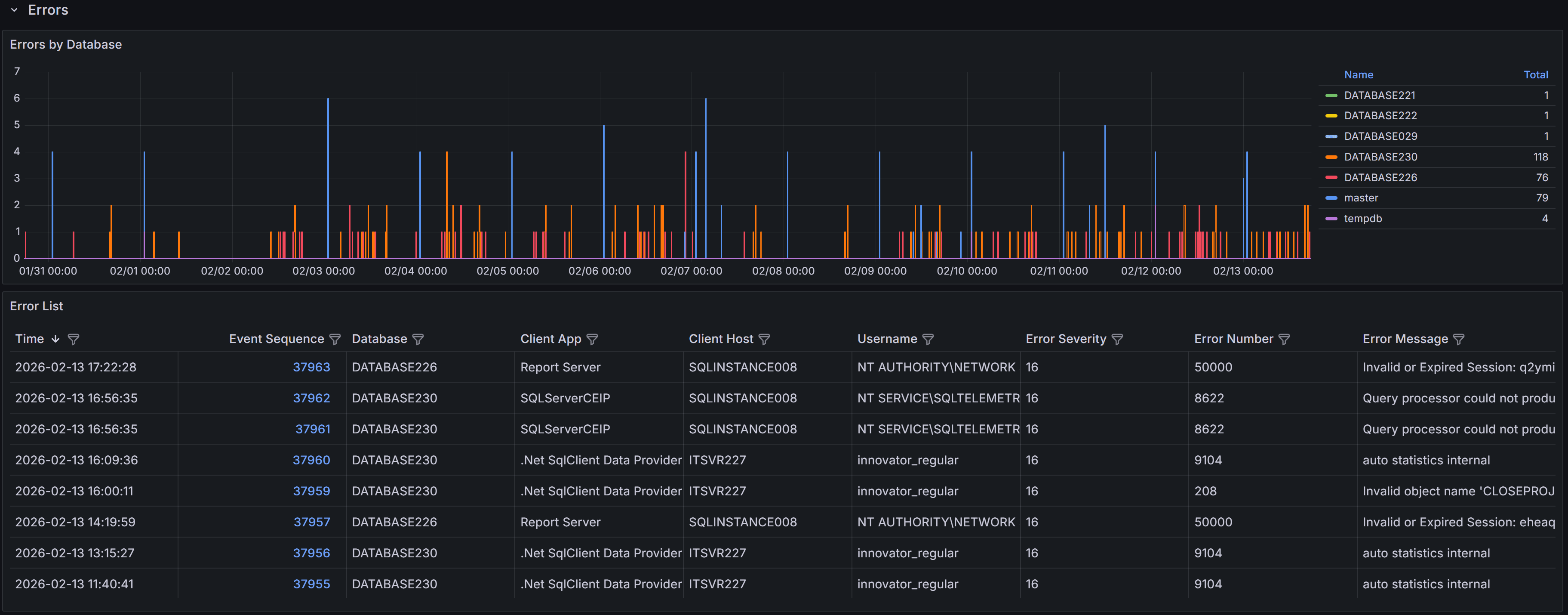Errors by database

Below the chart, a table lists individual error events with these columns:

• Time: the time the error occurred
• Event sequence: a unique identifier for the error event
• Database: Name of the database where the error occurred
• Client App: Name of the client application that caused the error
• Client Host: Name of the client host that originated the error
• Username: Login name of the connection where the error occurred
• Error Severity: the severity level of the error, on a scale from 16 to 25
• Error Number: the error number, which identifies the type of error
• Error Message: a brief description of the error

SQL Server error severity levels range from 0 to 25. This dashboard displays only errors with severity 16 or higher, which represent user-correctable errors and system-level problems. Severity 16-19 errors are typically application or query errors that users can fix. Severity 20-25 errors indicate serious system problems that may require DBA intervention. Understanding severity helps you prioritize which errors need immediate attention.

Error Details

Click the link in the Event Sequence column to open the error details dashboard. It shows the full error message and, when available, the SQL statement that caused the error. The SQL text may be unavailable for some error types.

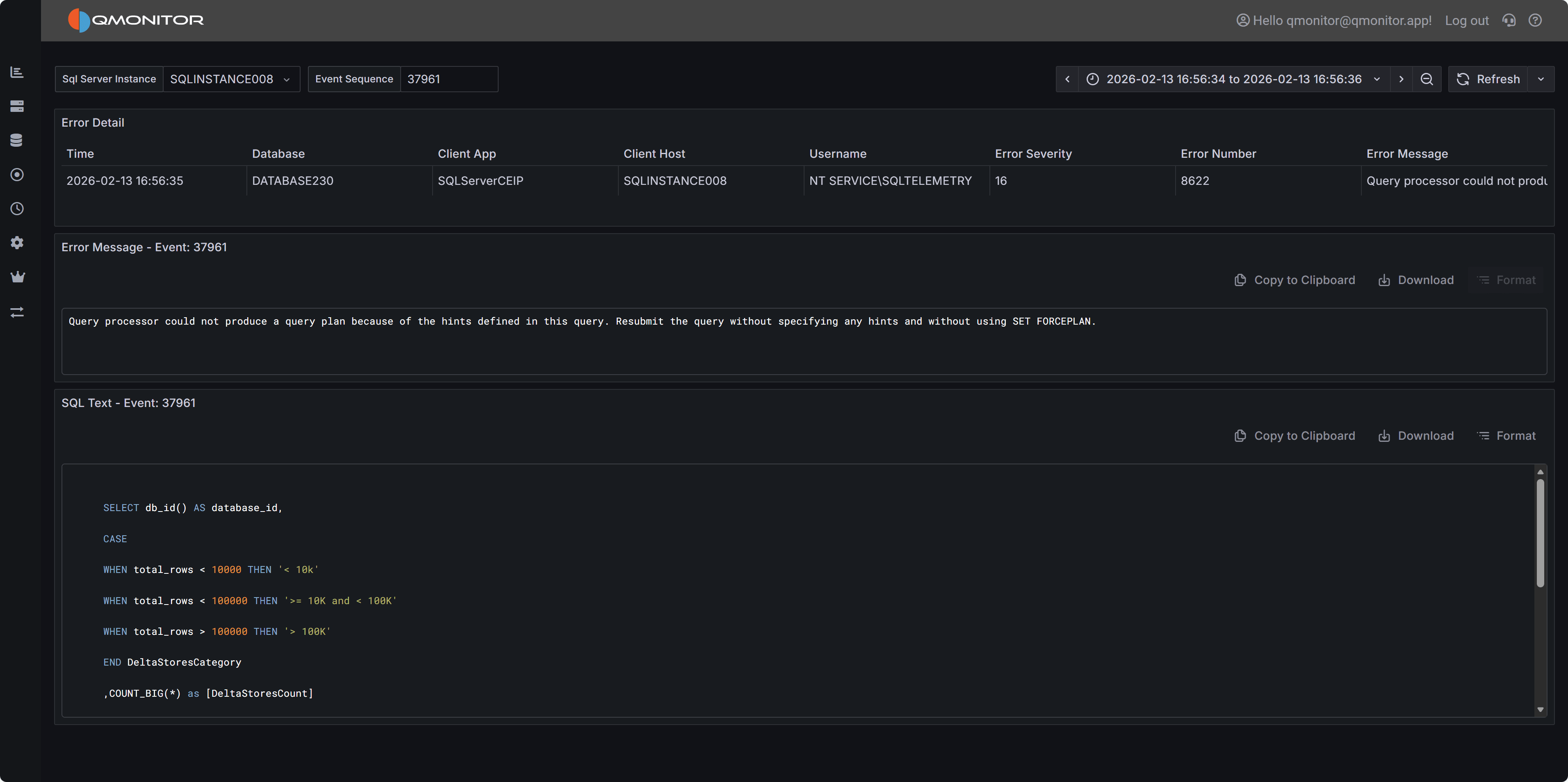Error Details

Common Error Patterns to Investigate

When analyzing errors, watch for these common patterns:

• Permission Errors (229, 297, 300, 15247) - Users attempting operations they don’t have rights to perform. Review permissions and ensure applications are using appropriate service accounts.

• Connection Errors (18456) - Failed login attempts. May indicate incorrect credentials, expired passwords, or potential security issues.

• Object Not Found (207, 208) - Queries referencing columns, tables, views, or procedures that don’t exist. Often occurs after deployments or when applications use wrong database contexts.

A complete list of SQL Server error numbers and their meanings can be found in the official documentation:

Using the Errors Dashboard Effectively

Start by filtering the time range to focus on recent errors or specific time periods when users reported issues. Use the database filter to focus on specific databases if you’re responsible for particular applications.

Filter by Error Number to display similar errors together. Grouping by error number helps you identify whether a single issue is affecting multiple users or databases.

When you find patterns of repeated errors, click through to the error details to examine the full error message and SQL statement. The SQL text often reveals the specific query or operation causing problems, allowing you to identify whether the issue is in application code, database schema, or data quality.

Monitor error trends over time by comparing different time periods. Increasing error rates may indicate degrading application quality, growing data volumes causing queries to fail, or infrastructure issues affecting database connectivity.

Exporting Error Events

You can export the error events table to CSV for offline analysis or sharing with development teams. Click on the three-dot menu in the table header and select Inspect –> Data to download the data in CSV format.

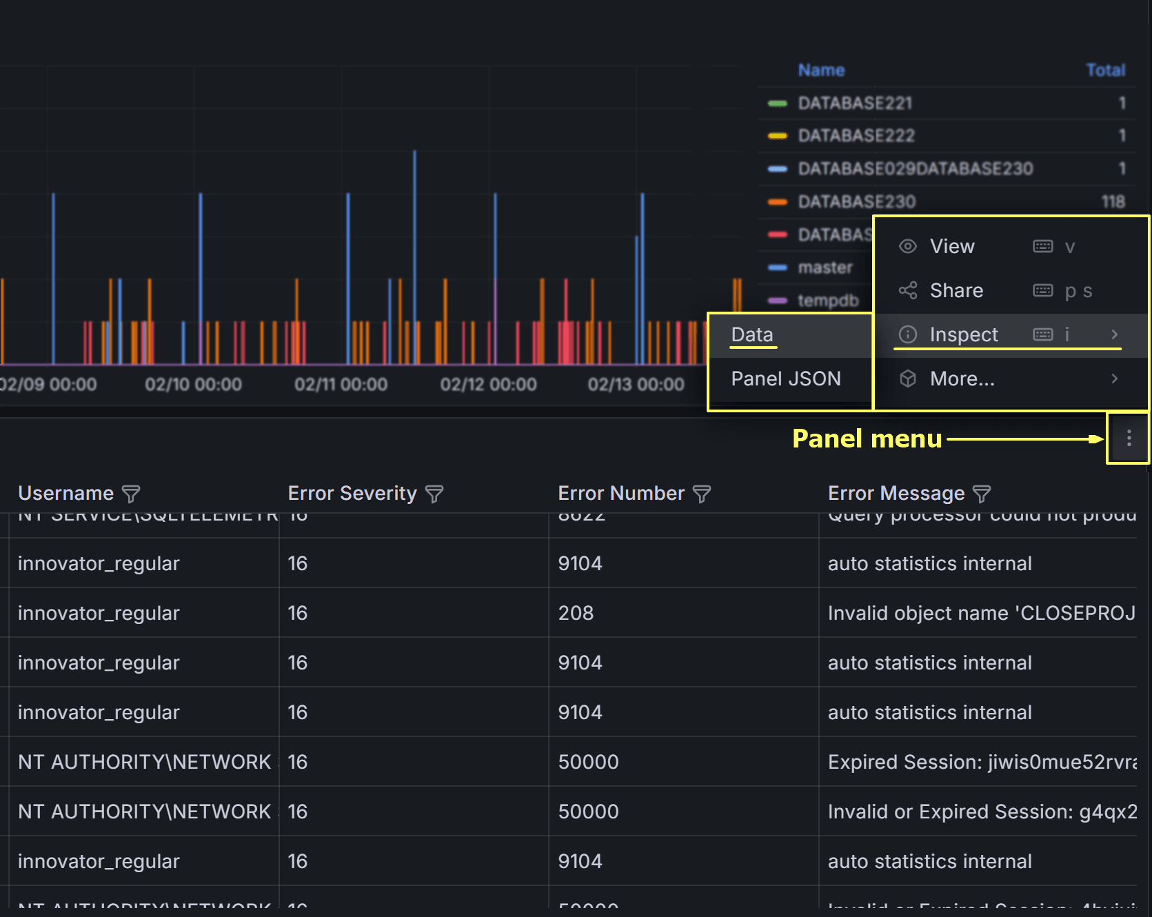
On the next dialog, make sure to check all three switches to download a result set that resembles the table view in the dashboard as closely as possible, including all columns and filters.

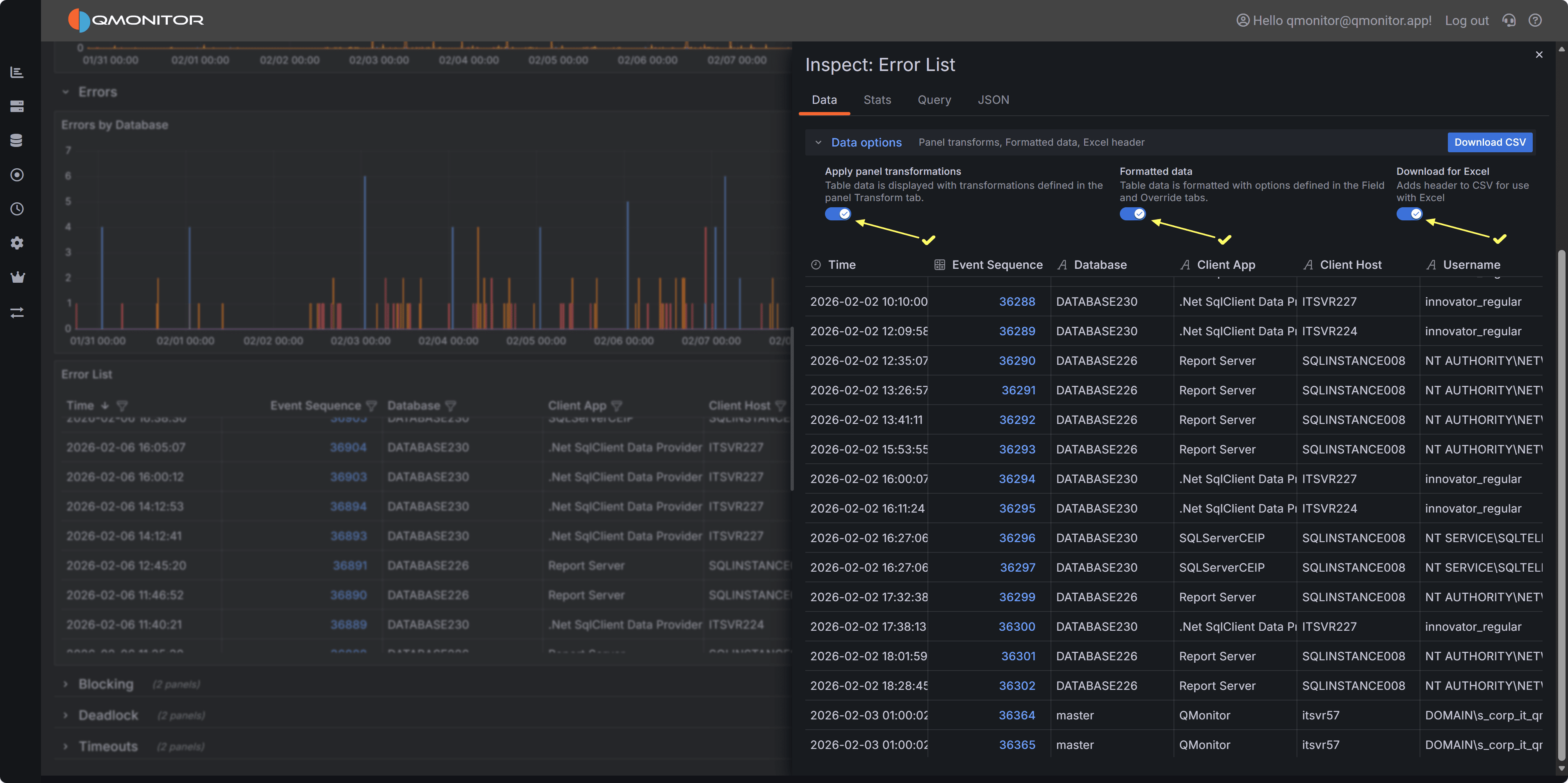
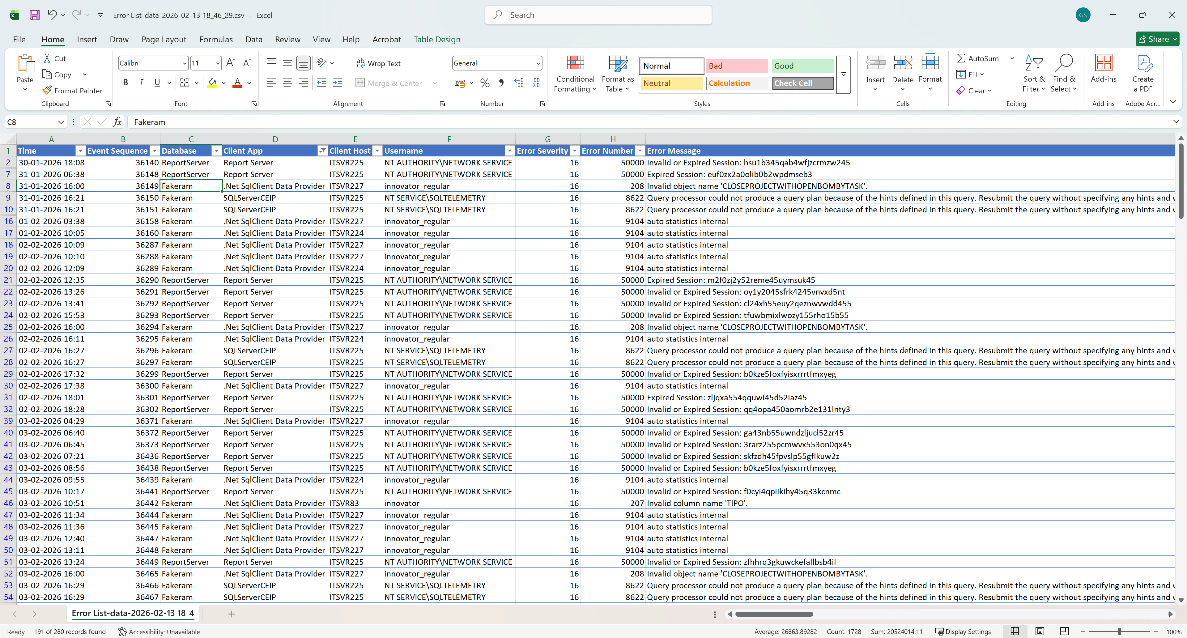
Click Download CSV to export the data. You can then open the CSV file in Excel or other tools for further analysis, such as pivoting by error number or database to identify common issues.

This is what the exported CSV file looks like when opened in Excel, with all columns and filters applied:

1.4.2 - Blocking

The Blocking dashboard helps you identify and diagnose sessions that are waiting for locks held by other sessions.

Understanding blocking patterns helps you identify problematic queries, optimize transaction design, and improve concurrency.

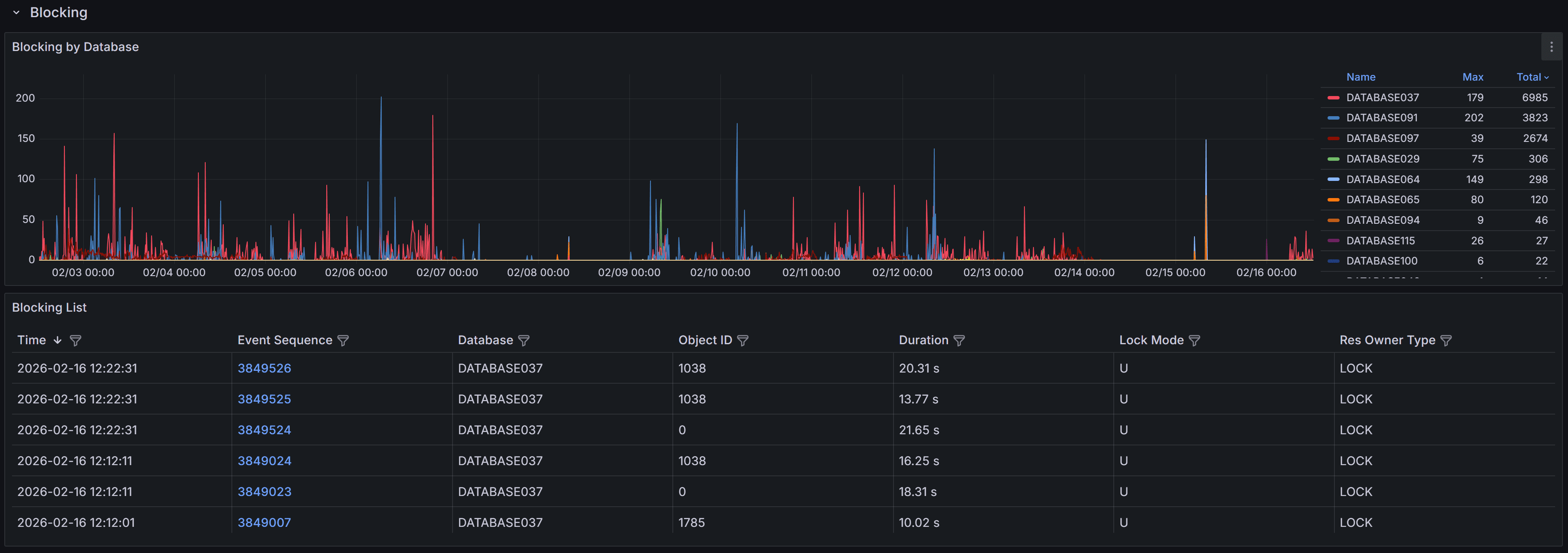
Expand the “Blocking” row to view a chart that shows the number of blocking events for each database.

SQL Server generates blocked process events only when a session waits on a lock longer than the configured blocked process threshold. By default, this threshold is set to 0 seconds, which means SQL Server does not generate blocking events at all.

The blocking events table below the chart provides detailed information about each blocking occurrence:

• Time shows when the blocking event was captured, helping you correlate blocking with other activities like batch jobs or peak usage periods.
• Event Sequence provides a unique identifier for the blocking event that you can reference when investigating or communicating with team members.
• Database identifies which database the blocking occurred in, helping you route investigation to the appropriate database owners.
• Object ID indicates the specific table or index involved in the lock, useful for identifying which database objects are causing contention.
• Duration displays how long the blocked session waited before the event was captured. Note that this is the wait time at the moment of capture; if blocking continued, the actual total wait time may be longer.
• Lock Mode shows the type of lock the blocking session holds (e.g., Exclusive, Shared, Update). Understanding lock modes helps you identify whether blocking is caused by writes blocking reads, writes blocking writes, or other lock compatibility issues.
• Resource Owner Type indicates what type of resource is being locked, such as a row, page, table, or database.

Use the column filters and sort controls to filter and sort the table.

Click a row to open the Blocking detail dashboard.

Blocking Event Details

When you click on a blocking event in the main table, the Blocking Detail dashboard opens with comprehensive information to help you diagnose the root cause.

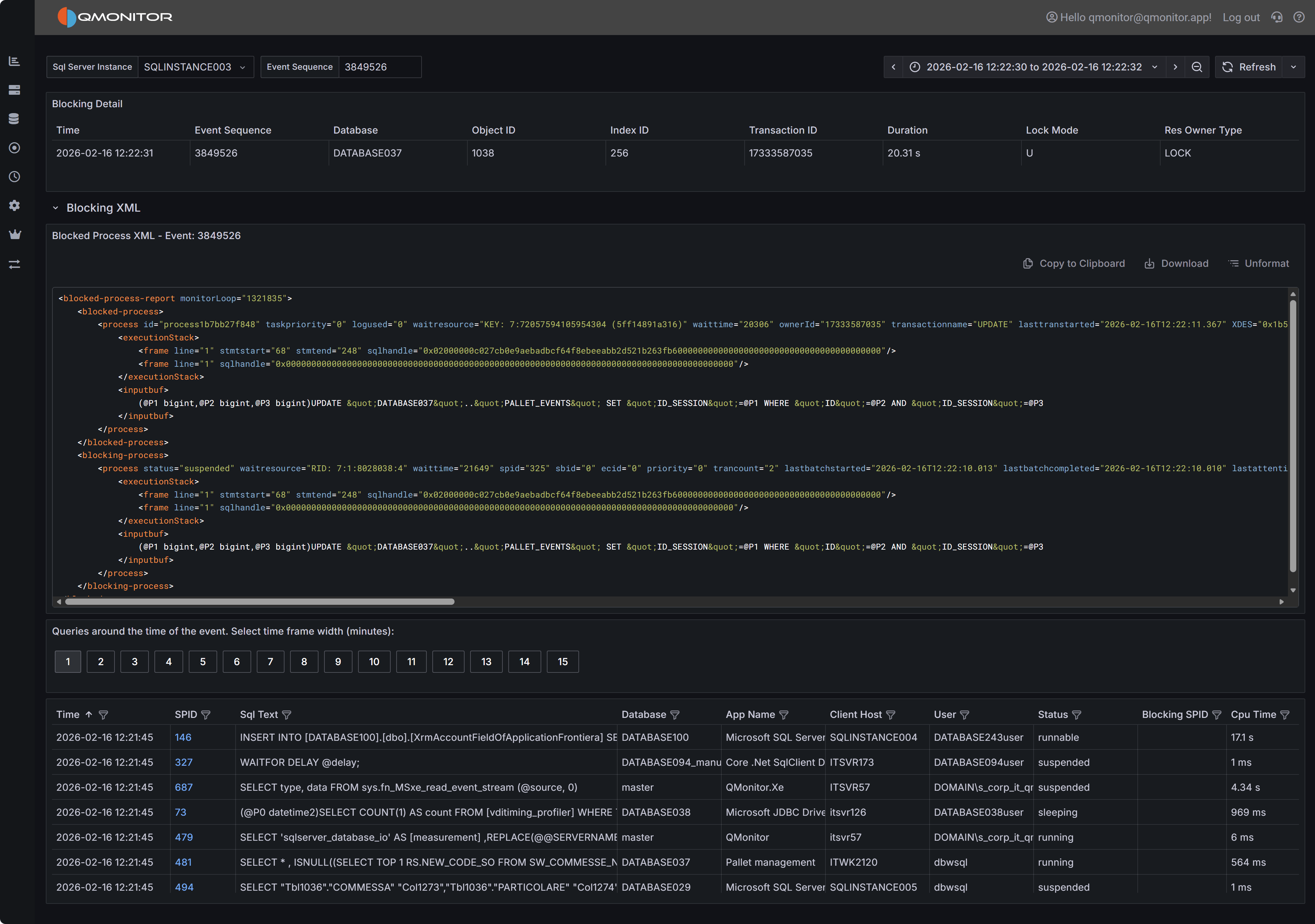Blocking event detail showing blocked and blocking processes

Event Summary

The top table provides key information about both the blocked and blocking processes. You’ll see the session IDs (SPIDs) of the blocked and blocking sessions, how long the blocking lasted, which database and object were involved, the lock mode causing the block, and the resource owner type. This summary gives you immediate context about what was blocked, what was blocking it, and how serious the impact was.

Blocked Process Report XML

The Blocked Process Report XML panel displays the complete XML report generated by SQL Server when the blocking event occurred. This XML contains detailed information about both the blocked and blocking sessions, including the SQL statements they were executing, their transaction isolation levels, and the specific resources they were waiting for or holding.

The XML includes one or more <blocked-process> nodes describing sessions that were waiting, and one or more <blocking-process> nodes describing sessions that held the locks. Each node contains attributes and child elements that provide:

• The SQL statement being executed (in the inputbuf element). This might be truncated if the statement is very long.
• The transaction isolation level
• Lock resource details (database ID, object ID, index ID, and the specific row or page being locked)
• The login name and host name of the session
• The current wait type and wait time

While the complete XML schema is documented in Microsoft’s SQL Server documentation, the most immediately useful information is typically the SQL text from both the blocked and blocking processes. Documenting the complete XML structure is beyond the scope of this documentation.

Active Sessions Grid

The bottom grid lists all sessions that were active around the time the blocking event occurred. This context is valuable because blocking chains often involve multiple sessions, and understanding the overall session activity helps you identify patterns and root causes.

Use the time window buttons above the grid to adjust how far before and after the blocking event you want to see session data. Options range from 1 minute to 15 minutes. A wider window provides more context but may include unrelated sessions.

1.4.3 - Deadlocks

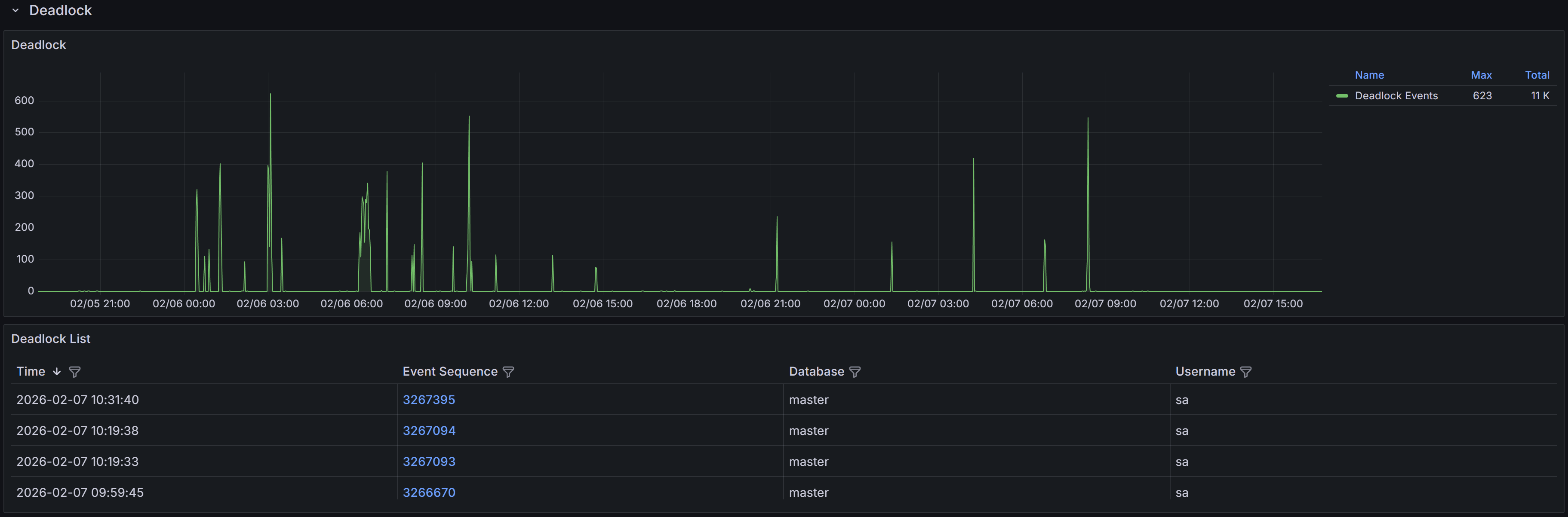
The Deadlocks dashboard helps you identify and diagnose deadlock situations.

Expand the “Deadlocks” row to view a chart that shows the number of deadlocks for each database.

Understanding Deadlocks

A deadlock occurs when two or more sessions create a circular dependency on locks.

SQL Server’s deadlock detector runs every few seconds to identify these circular lock dependencies. When a deadlock is detected, SQL Server analyzes the sessions involved and chooses one as the “deadlock victim” based on factors like transaction cost and deadlock priority. The victim’s current statement is rolled back with error 1205, while other sessions proceed normally. The application that receives error 1205 should catch this error and retry the transaction, as the same operation will typically succeed on retry once the competing transaction completes.

QMonitor captures deadlock events through SQL Server extended events and stores the complete deadlock graph as XML. This graph contains detailed information about all sessions involved in the deadlock, the resources they were competing for, and the SQL statements they were executing at the time.

The deadlock events table below the chart lists all captured deadlocks with the following information:

• Time shows when the deadlock occurred, helping you identify patterns such as deadlocks during batch processing or peak usage periods.
• Event Sequence provides a unique identifier for the deadlock event that you can use when communicating with team members or referencing in tickets.
• Database identifies which database the deadlock occurred in, helping you route investigation to the appropriate database owners and application teams. This is often reported as “master”,
• but the graph itself contains the actual database context for each session.
• User Name shows the SQL Server login involved in the deadlock, useful for identifying which applications or users are experiencing deadlock issues.

Use the column filters to narrow the list to specific databases or time periods, and sort by Time to see the most recent deadlocks first or to identify clusters of deadlocks occurring in quick succession.

Click a row to open the Deadlock detail dashboard.

Deadlock Event Details

When you click on a deadlock event in the main table, the Deadlock Detail dashboard opens with comprehensive information to help you understand and resolve the deadlock.

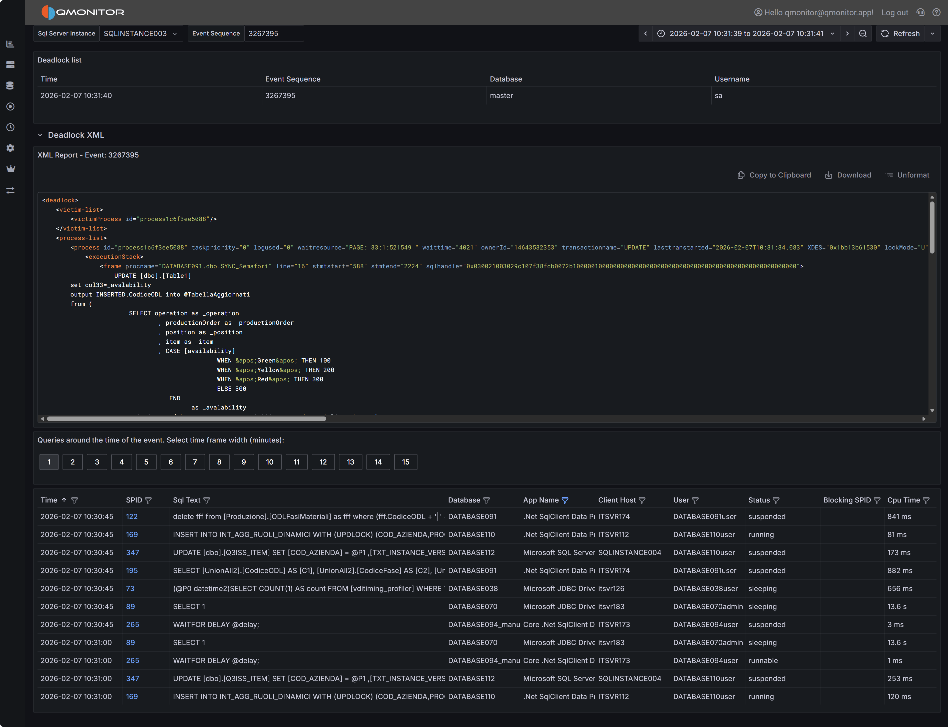Deadlock event detail showing deadlock graph XML and active sessions

Deadlock Graph XML

The deadlock graph XML panel displays the complete XML representation of the deadlock as captured by SQL Server. This XML contains all the information SQL Server used to detect and resolve the deadlock, making it the authoritative source for understanding what happened.

The XML structure includes several key node types:

Process Nodes (<process>) describe each session involved in the deadlock. Each process node contains:

• The session ID (SPID) and transaction ID
• Whether the process was chosen as the deadlock victim
• The isolation level the transaction was using
• Lock mode and lock request mode
• The SQL statement being executed (in the <inputbuf> element)
• The execution stack showing which stored procedures or code paths led to the deadlock

Resource Nodes describe the database objects involved in the deadlock, such as:

• <keylock> for row-level locks on index keys
• <pagelock> for page-level locks
• <objectlock> for table-level locks
• <ridlock> for row identifier locks on heap tables

Each resource node shows which processes own locks on the resource and which processes are waiting for locks on that resource, revealing the circular dependency.

Owner and Waiter Lists within each resource node show the lock ownership chain. By following the owners and waiters across resources, you can trace the deadlock cycle: Process A owns Resource 1 and waits for Resource 2, while Process B owns Resource 2 and waits for Resource 1.

Reading the Deadlock Graph

To analyze a deadlock, start by identifying the victim process (marked with deadlock-victim="1" in the process node). Then examine the SQL statements in all participating processes to understand what operations were attempting to execute.

Look at the resource nodes to identify which database objects were involved. The object names are typically shown as object IDs that you can look up in sys.objects, but the associated index IDs and database names provide immediate context.

Trace the lock ownership chain by following the <owner-list> and <waiter-list> elements. This reveals the exact sequence of lock requests that formed the deadlock cycle. Understanding this sequence is crucial for determining how to prevent the deadlock.

Pay attention to the isolation levels shown in the process nodes. Higher isolation levels like REPEATABLE READ or SERIALIZABLE hold locks longer and increase deadlock likelihood. If you see these isolation levels, consider whether they’re truly necessary for the business logic.

Active Sessions Context

The bottom grid shows sessions that were active around the time the deadlock occurred. Use the time window buttons (1 to 15 minutes) to expand or narrow the view.

This context helps you understand the overall workload and identify whether there were other related activities occurring simultaneously. For example, if you see multiple similar queries running at the same time, this might indicate that concurrency issues need to be addressed at the application level through better transaction design or job scheduling.

1.4.4 - Timeouts

The Timeouts dashboard helps you identify and diagnose queries that exceed their configured timeout limits before completing execution. Query timeouts occur when the time required to execute a query exceeds the timeout value set by the client application, connection string, or command object. When a timeout occurs, the client cancels the query and typically returns an error to the user.

Expand the “Timeouts” row to view a chart that shows the number of timeouts for each database.

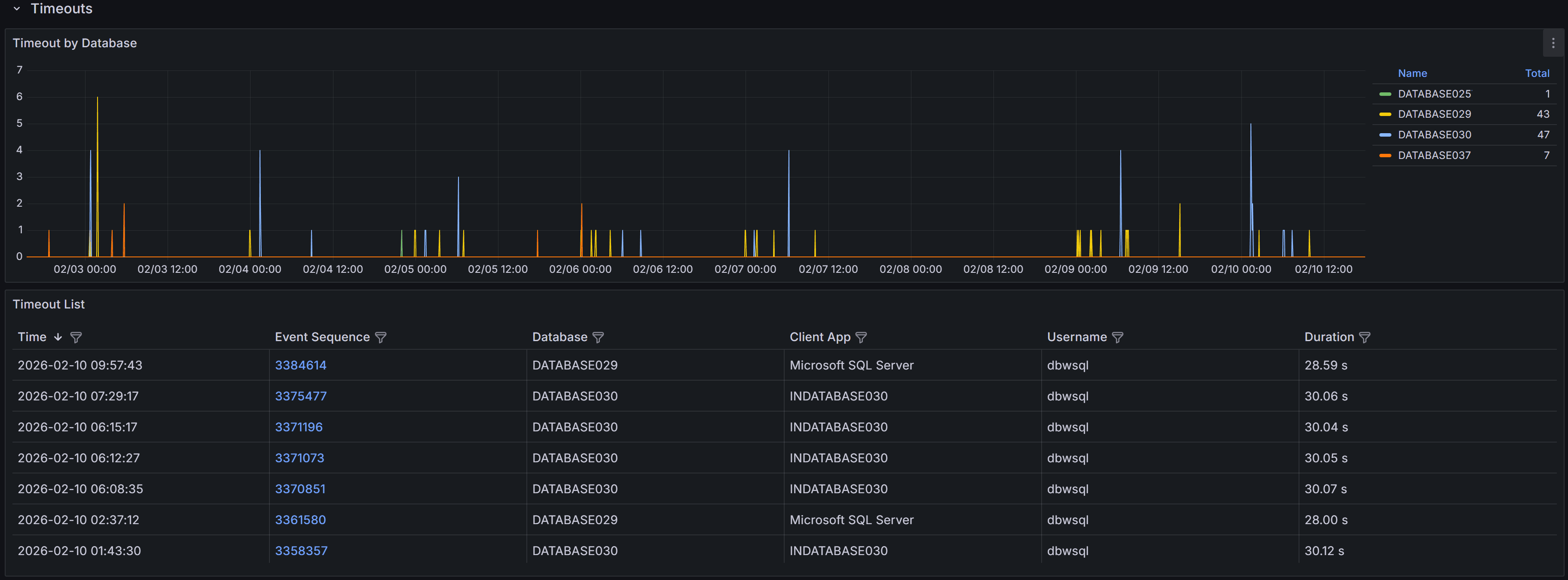
QMonitor captures timeout events and records the error text, session details, and, when available, the SQL text.

The timeout events table below the chart provides detailed information about each timeout occurrence:

• Time shows when the timeout occurred, helping you correlate timeouts with other activities such as batch jobs, report generation, or peak usage periods.
• Event Sequence provides a unique identifier for the timeout event that you can reference when investigating or communicating with team members.
• Database identifies which database the timed-out query was executing against, helping you route investigation to the appropriate database owners.
• Duration shows how long the query had been running when it timed out. This is crucial information: if duration is close to common timeout values (30, 60, or 120 seconds), the timeout setting may be appropriate and the query needs optimization. If duration is much shorter, there may have been network issues or the client may have cancelled prematurely.
• Application displays the application name from the connection string, helping you identify which applications or services are experiencing timeout issues.
• Username shows the SQL Server login used for the connection, useful for identifying whether timeouts are widespread or isolated to specific users or service accounts.

Use the column filters to focus on specific databases or applications, and sort by Duration to identify whether timeouts are occurring at consistent durations (suggesting timeout setting issues) or varying durations (suggesting query performance problems).

Timeout Event Details

When you click on a timeout event in the main table, the Timeout Detail dashboard opens with comprehensive information to help you diagnose the root cause.

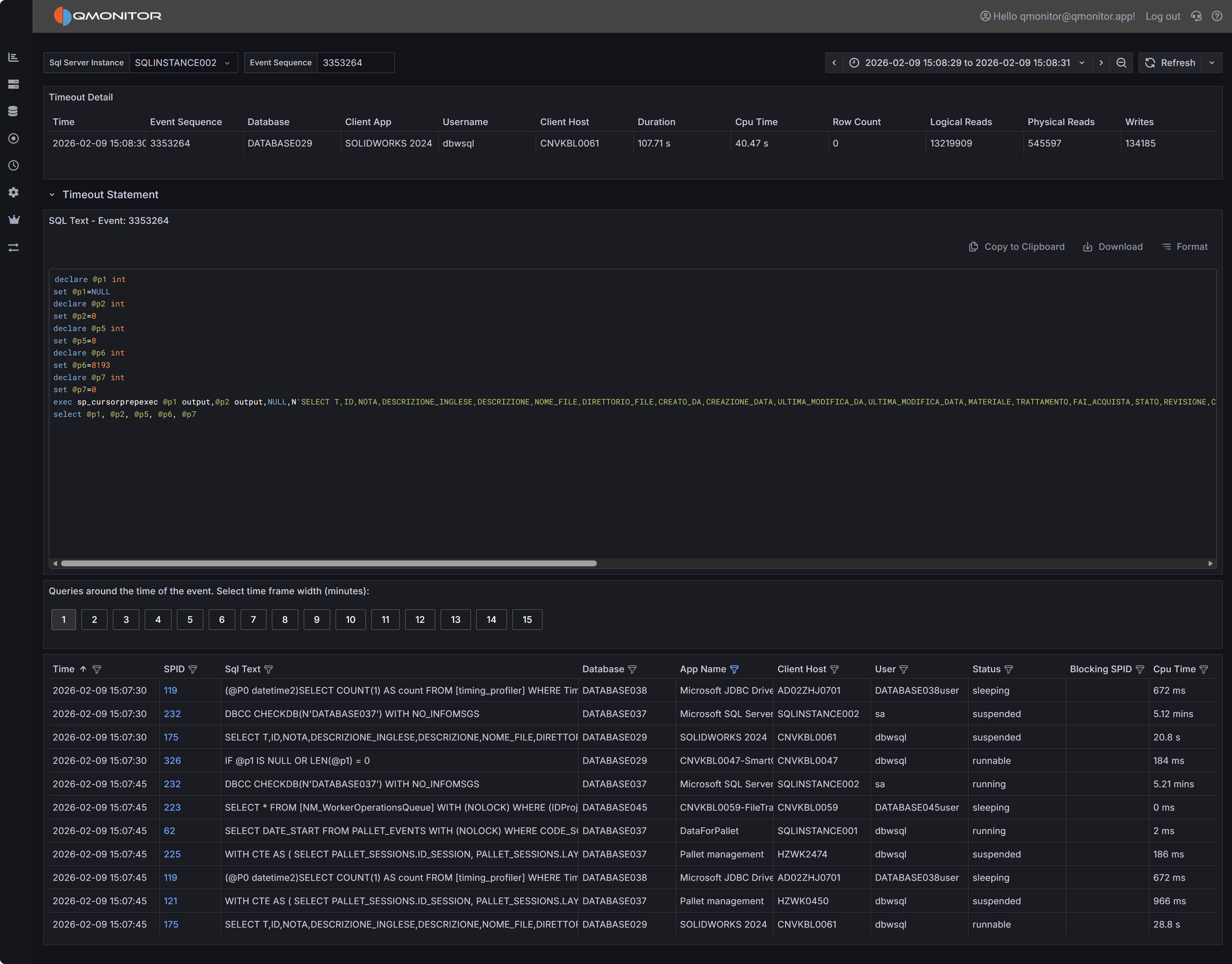Timeout event detail showing event summary, SQL statement, and active sessions

Event Summary

The top table displays key information about the timeout event, including the exact time it occurred, the database involved, the duration before timeout, the application name, and the username. This summary gives you immediate context about the circumstances of the timeout.

SQL Statement

The SQL Statement panel displays the query that timed out, when this information is available. Having the complete SQL text is essential for investigating whether the query itself needs optimization. You can copy this text to run the query in SQL Server Management Studio with execution plans enabled to identify expensive operators, missing indexes, or inefficient query patterns.

Note that SQL text may not be available for all timeout events. Some timeouts occur during connection establishment or for system operations that don’t have associated SQL text. When SQL text is unavailable, focus on the session context and timing to understand what was happening.

Active Sessions Context

The bottom grid shows all sessions that were active around the time the timeout occurred. This context is useful for understanding whether the timeout was an isolated incident or part of broader performance issues affecting the instance.

Use the time window buttons above the grid to adjust the view from 1 to 15 minutes before and after the timeout. A wider window provides more context about overall instance activity, while a narrower window focuses specifically on sessions active during the timeout.

Look for patterns in the active sessions grid:

• Blocking chains where multiple sessions are waiting on locks held by others, which may have delayed your timed-out query
• Resource-intensive queries running concurrently that may have caused CPU or I/O contention
• Similar queries running simultaneously, indicating potential concurrency issues at the application level
• Long-running transactions that might be holding locks or consuming resources

Filter the grid to show only blocked sessions or sessions with high CPU or I/O metrics to quickly identify potential causes of the timeout.

1.5 - SQL Server I/O Analysis

The SQL Server I/O Analysis dashboard provides comprehensive visibility into disk I/O performance across your SQL Server instance. Understanding I/O patterns and performance is essential for diagnosing storage bottlenecks, capacity planning, and optimizing query performance. This dashboard breaks down I/O metrics by volume, database, and file type, helping you identify where I/O resources are being consumed and whether storage performance meets workload requirements.

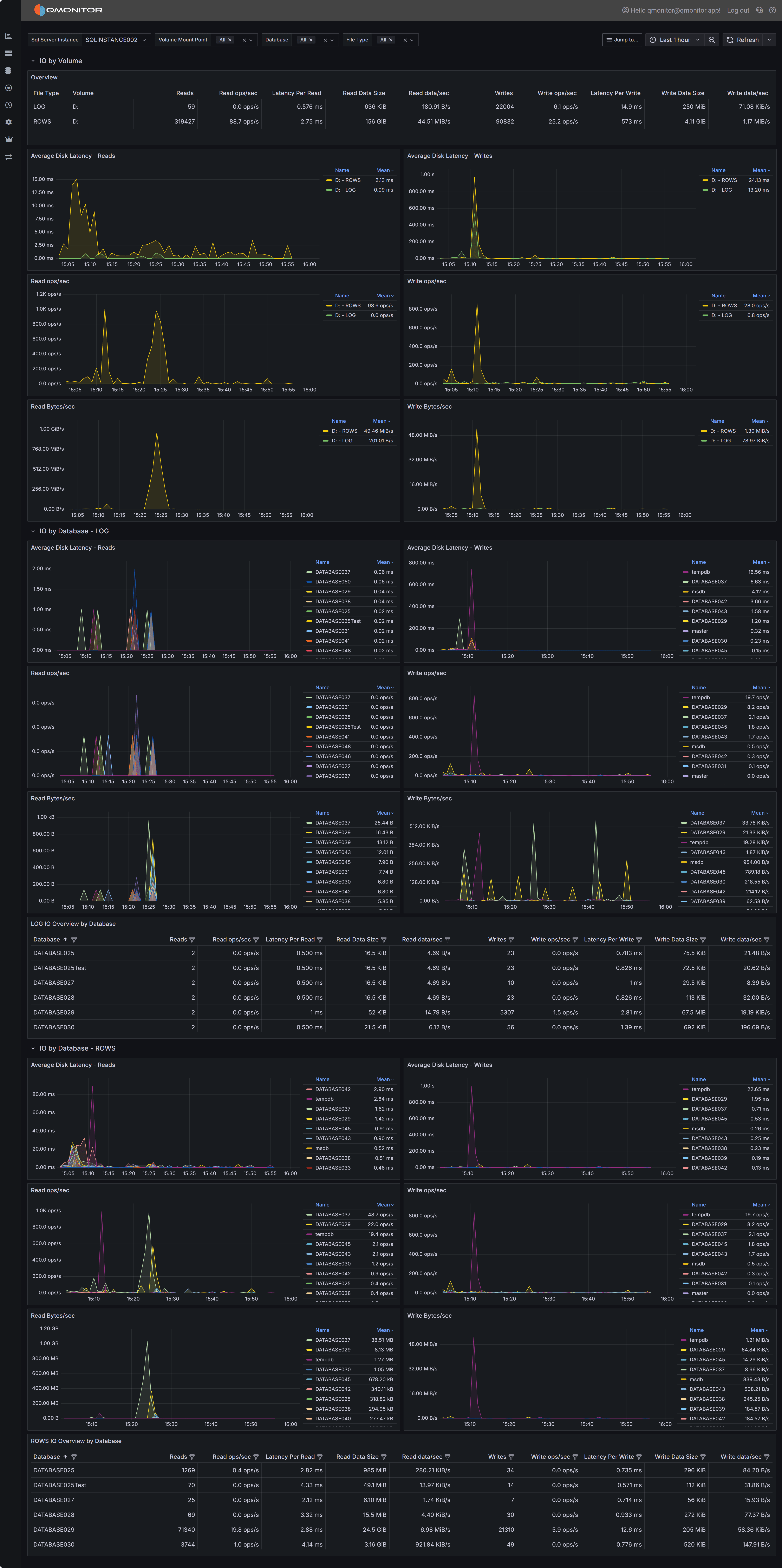SQL Server I/O Analysis dashboard showing I/O metrics by volume and database

Dashboard Sections

I/O by Volume

The I/O by Volume section provides an overview of disk I/O performance at the volume level, showing how each physical or logical volume hosting SQL Server data and log files is performing.

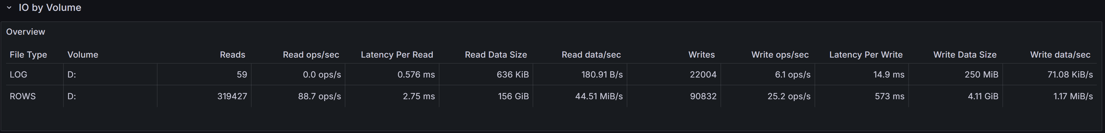
Overview Table

The overview table displays key I/O metrics for each volume:

• File Type indicates whether the volume contains data files (ROWS) or log files (LOG). This distinction is important because data and log files have different I/O patterns: data files typically have mixed random and sequential I/O, while log files have predominantly sequential write I/O.
• Volume shows the drive letter or mount point where SQL Server files reside.
• Reads displays the total number of read operations performed on this volume during the selected time range. High read counts on data volumes may indicate memory pressure forcing SQL Server to read from disk frequently, or queries performing large scans.
• Read ops/sec shows the average read operations per second, indicating read workload intensity.
• Latency Per Read displays the average time in milliseconds for read operations to complete. For modern SSD storage, read latency should typically be under 5ms. Latencies above 10ms may indicate storage performance issues, excessive load, or storage configuration problems.
• Read Data Rate shows the throughput in MB/s for read operations, indicating how much data is being read from the volume per second.
• Read stalls/sec indicates how frequently read operations are delayed waiting for I/O completion. High stall rates combined with high latency suggest storage performance problems.
• Writes displays the total number of write operations performed on this volume.
• Write ops/sec shows the average write operations per second.
• Latency Per Write displays the average time in milliseconds for write operations to complete. Write latency is typically higher than read latency, but values consistently above 20ms may indicate problems.
• Write Data Rate shows the throughput in MB/s for write operations.
• Write stalls/sec indicates how frequently write operations are delayed.

Use this table to identify volumes with high latency or stall rates that may be experiencing performance problems. Compare read and write patterns to understand whether volumes are primarily serving read-heavy or write-heavy workloads.

I/O Performance Charts

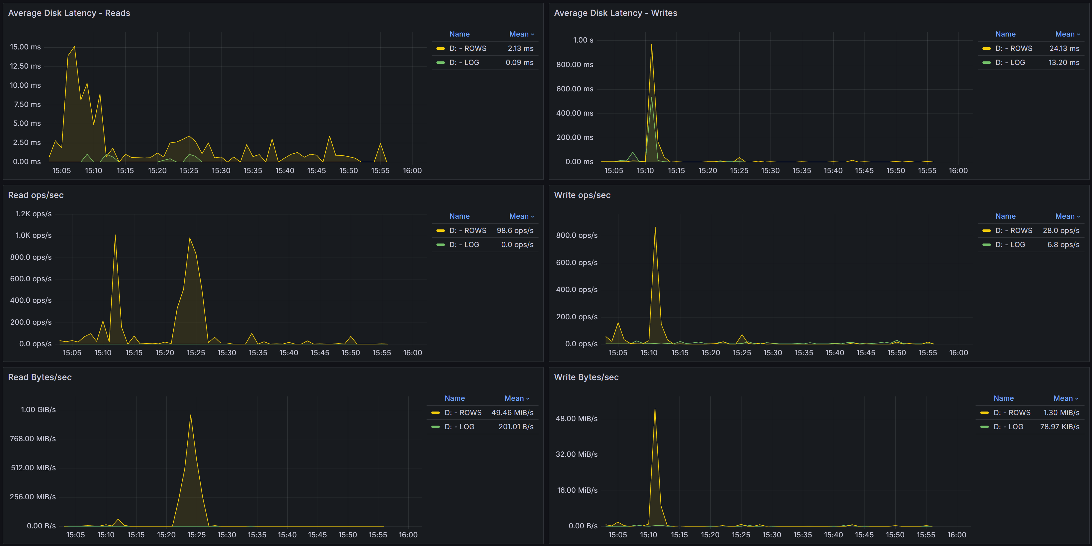
Below the overview table, several charts visualize I/O performance trends over time:

Average Disk Latency - Reads shows how read latency varied during the selected time period for each volume. Spikes in read latency often correlate with periods of high concurrent query activity, memory pressure forcing more physical reads, or storage system performance issues. Consistent high latency suggests chronic storage performance problems that need investigation.

Average Disk Latency - Writes displays write latency trends. For log file volumes, write latency directly impacts transaction commit times since transactions cannot complete until log writes finish. High or spiking write latency on log volumes can significantly impact application performance.

Read ops/sec charts show read operation intensity over time. Sudden increases in read operations may indicate new queries, missing indexes forcing table scans, or decreased buffer cache hit ratios due to memory pressure or cache churn.

Write ops/sec charts display write operation intensity. Write spikes often correlate with checkpoint activity, index maintenance operations, large data modifications, or log activity during high transaction volumes.

Read Bytes/sec shows read throughput over time. High read throughput with many read operations suggests random I/O patterns, while high throughput with fewer operations indicates large sequential reads.

Write Bytes/sec displays write throughput trends. For data files, write throughput reflects checkpoint activity and dirty page flushing. For log files, it reflects transaction log write activity.

I/O by Database - LOG

The I/O by Database - LOG section breaks down log file I/O performance by individual database, helping you identify which databases generate the most transaction log activity.

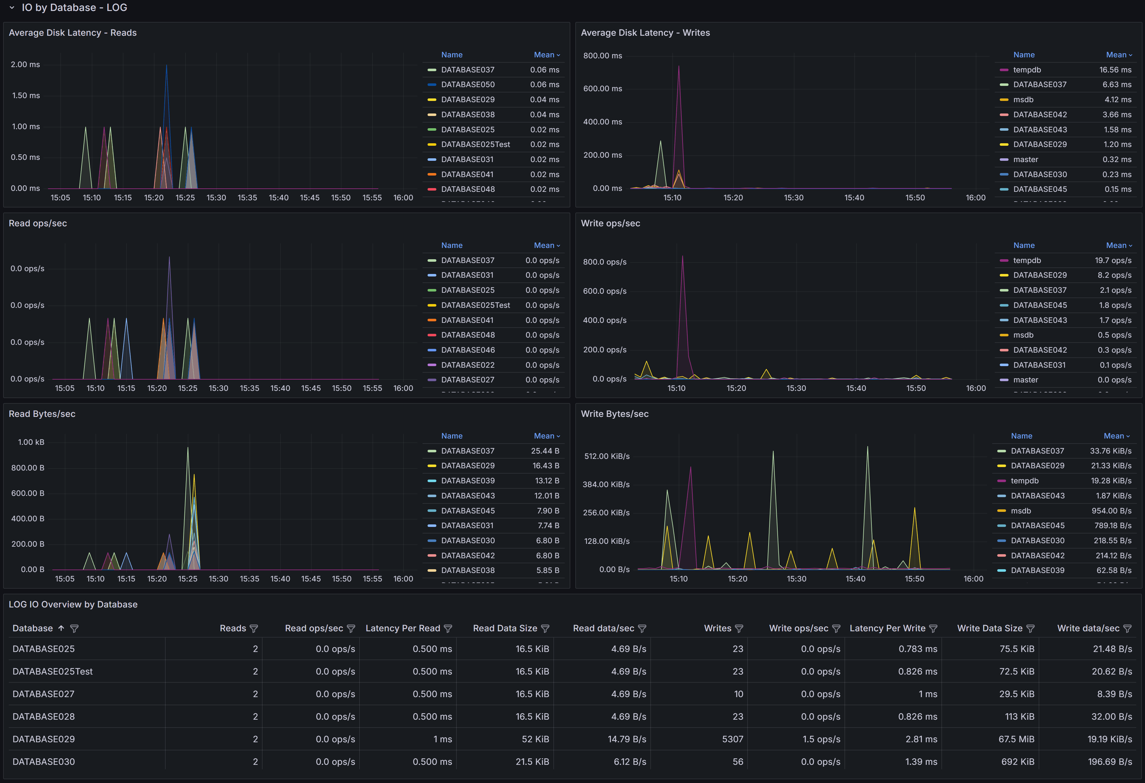
Log I/O Metrics Table

The table displays detailed log file I/O metrics for each database:

• Database identifies the database name.
• Reads shows the number of read operations on the transaction log. Log reads occur during operations like transaction rollback, database recovery, or transaction log backups. High log read activity outside of these scenarios is unusual and may indicate problems.
• Read ops/sec indicates the rate of log read operations.
• Latency Per Read shows average log read latency. Log reads are typically infrequent, but high latency can impact recovery operations.
• Read Data Rate displays log read throughput.
• Read stalls/sec shows how often log reads are delayed.
• Writes displays the total number of log write operations. Every transaction that modifies data must write to the transaction log, making this a key metric for understanding database activity.
• Write ops/sec shows the rate of log write operations, which correlates directly with transaction throughput.
• Latency Per Write is one of the most critical I/O metrics. Log writes are synchronous: transactions cannot commit until their log records are written to disk. High log write latency directly impacts transaction throughput and application performance. Values above 10-15ms may significantly impact user experience.
• Write Data Rate shows log write throughput, indicating how much transaction log data is being generated per second.
• Write stalls/sec indicates how often log write operations are delayed waiting for I/O completion.

Log I/O Performance Charts

The charts visualize log I/O trends for each database:

Average Disk Latency - Reads shows log read latency trends. Spikes during backup operations are normal.

Average Disk Latency - Writes is critical for understanding transaction performance. Consistent high write latency indicates storage problems affecting transaction commit times.

Read ops/sec and Write ops/sec charts show log I/O activity patterns. Write operations should correlate with transaction activity patterns: high during business hours, lower during off-peak times.

Read Bytes/sec and Write Bytes/sec show log throughput trends. High log write throughput indicates heavy transaction activity or large data modifications.

I/O by Database - ROWS

The I/O by Database - ROWS section breaks down data file I/O performance by database, showing which databases consume the most data file I/O resources.

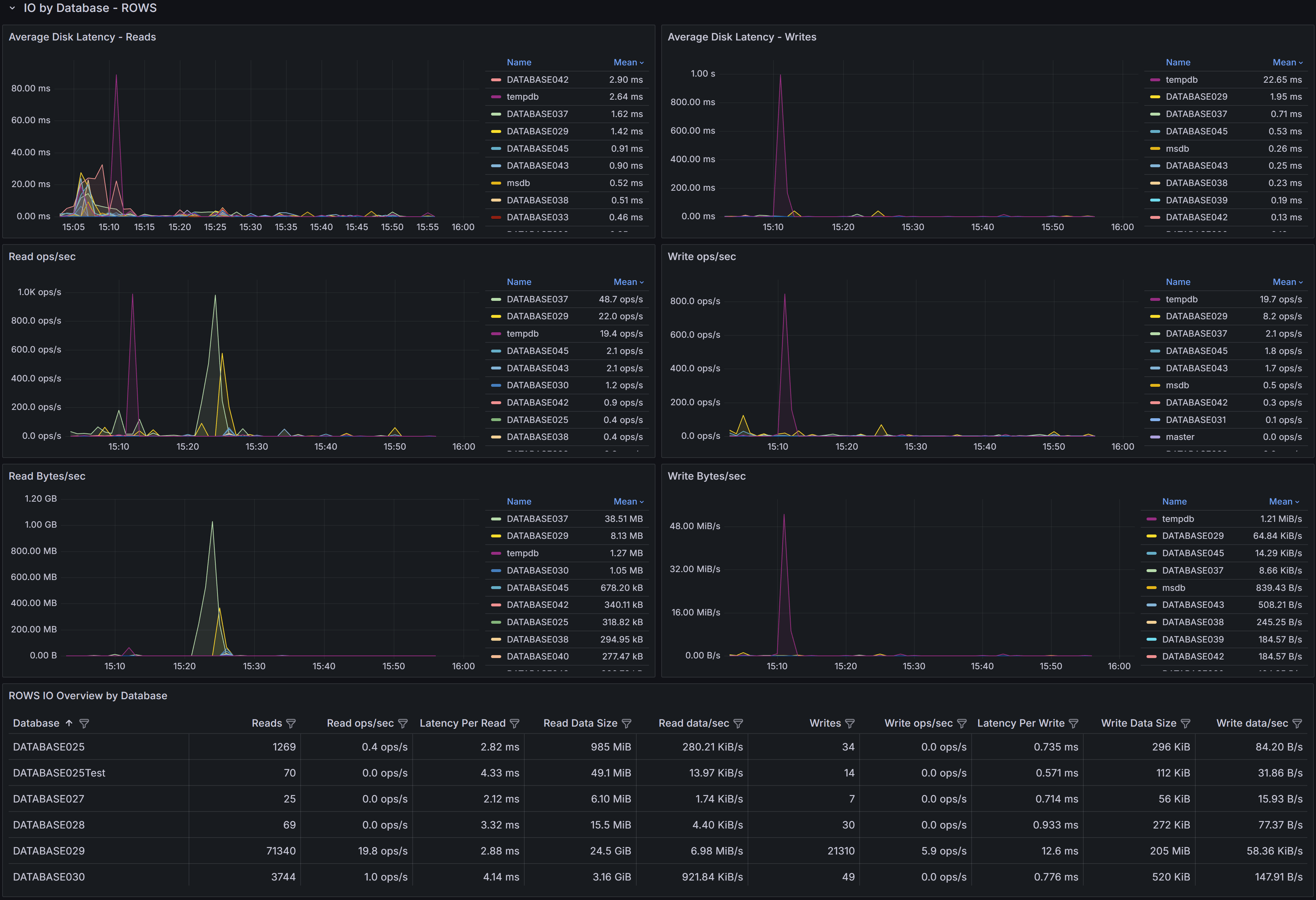
Data File I/O Metrics Table

The table displays comprehensive data file I/O metrics:

• Database identifies the database name.
• Reads shows the total read operations on data files. High read counts may indicate memory pressure, missing indexes causing table scans, or queries retrieving large result sets.
• Read ops/sec indicates read operation intensity.
• Latency Per Read shows average data file read latency. High latency impacts query performance, especially for queries that must read from disk frequently due to insufficient memory or inefficient execution plans.
• Read Data Rate displays data file read throughput.
• Read stalls/sec shows how often read operations are delayed.
• Writes displays data file write operations. Writes occur during checkpoint operations when dirty pages are flushed to disk, during lazy writer activity, and during certain operations like SELECT INTO or bulk inserts.
• Write ops/sec shows write operation rate.
• Latency Per Write indicates how long write operations take to complete. While data file writes are typically asynchronous (unlike log writes), high write latency can still impact performance by preventing SQL Server from freeing up buffer pool memory for new pages.
• Write Data Rate shows data file write throughput.
• Write stalls/sec indicates write operation delays.

Data File I/O Performance Charts

The charts visualize data file I/O trends:

Average Disk Latency - Reads shows how read latency varies over time. Spikes often correlate with concurrent query activity, memory pressure, or queries performing large scans. Use this chart with the Memory section of the Instance Overview dashboard to understand whether high read latency is related to insufficient buffer cache.

Average Disk Latency - Writes displays write latency trends for data files. Spikes during checkpoint intervals are normal, but consistently high latency may indicate storage performance issues.

Read ops/sec charts show data file read activity. Compare these patterns with query execution patterns to understand whether high reads correlate with specific queries or time periods.

Write ops/sec charts display write activity patterns. Regular spikes typically correspond to checkpoint intervals configured for your instance.

Read Bytes/sec and Write Bytes/sec show data file throughput trends, helping you understand I/O bandwidth consumption patterns.

Interpreting I/O Metrics

Understanding what I/O metrics reveal about your system is essential for effective troubleshooting and optimization.

High Read Latency on Data Files typically indicates one of several issues: storage system performance problems, excessive concurrent I/O load exceeding storage capacity, memory pressure forcing more physical reads than the storage can efficiently handle, or storage configuration issues like improper RAID levels or insufficient disk spindles. Compare read latency trends with memory metrics from the Instance Overview dashboard: if Page Life Expectancy is low and read latency is high, adding memory may be more effective than upgrading storage.

High Write Latency on Log Files is particularly critical because it directly impacts transaction commit times and application performance. Potential causes include storage system limitations, log files on slow storage or shared with other I/O intensive workloads, write caching disabled or improperly configured, or network latency if using SAN storage. Even a few milliseconds of improvement in log write latency can significantly impact transaction throughput.

High Read Operations/sec may indicate memory pressure causing poor buffer cache hit ratios, missing indexes forcing table scans that read many pages, queries retrieving large result sets, or increased workload. Investigate whether query optimization or memory increases would be more effective than storage upgrades.

High Write Operations/sec on data files often reflects checkpoint activity flushing dirty pages. If write spikes correlate with checkpoint intervals, this is normal behavior. If writes are consistently high, investigate whether large index maintenance operations, bulk data loads, or heavy UPDATE/DELETE activity is occurring.

Stalls indicate I/O operations delayed waiting for storage. High stall rates combined with high latency clearly indicate storage performance problems. Even with acceptable average latency, high stall rates suggest inconsistent storage performance that may impact user experience.

Using the Dashboard for Troubleshooting

When investigating storage-related performance problems, start with the I/O by Volume section to identify which volumes are experiencing high latency or stall rates. This helps you determine whether problems are isolated to specific volumes or affect all storage.

If log file volumes show high write latency, this should be your top priority because it directly impacts every transaction. Log writes are synchronous, so improving log write performance can yield immediate benefits for transaction throughput. Consider moving log files to faster storage, enabling write caching if safe, or investigating whether multiple databases’ log files are competing for resources on the same volume.

Check whether data file I/O problems are widespread across all databases or isolated to specific databases. If isolated, focus optimization efforts on those databases through query tuning, indexing, or memory allocation. If widespread, consider storage upgrades or instance-level memory increases.

Compare I/O patterns with other dashboard data. High read operations with low Page Life Expectancy suggests memory pressure. High read operations with missing index warnings in query plans suggests index optimization opportunities. High I/O during specific time windows suggests investigating what workloads run during those periods.

Use the time range selector to compare current I/O metrics with historical baselines. Gradually increasing latency over time may indicate growing data volumes exceeding storage capacity, while sudden latency increases suggest configuration changes, new workloads, or storage system problems.

Storage Optimization Strategies

Based on I/O analysis findings, consider these optimization approaches:

Separate Workloads - Place log files on separate physical storage from data files. Log file I/O is sequential and latency-sensitive, while data file I/O is mixed random and sequential. Separating them prevents interference and allows tuning storage for each workload’s characteristics.

Use Faster Storage for Logs - Since log write latency directly impacts transaction throughput, placing log files on the fastest available storage (NVMe SSDs, for example) provides immediate performance benefits. Even modest log write latency improvements can significantly increase transaction throughput.

Enable Write Caching - On storage controllers with battery-backed or flash-backed cache, enable write caching for log file volumes. This can dramatically reduce log write latency. Ensure proper backup power protection to prevent data loss.

Increase Memory - Before upgrading storage, evaluate whether increasing SQL Server memory would reduce I/O load by improving buffer cache hit ratios. More memory means fewer reads from disk, potentially eliminating the need for storage upgrades.

Optimize Queries and Indexes - High I/O volumes caused by inefficient queries or missing indexes are best solved through query optimization rather than storage upgrades. Use the Query Stats dashboard to identify high-I/O queries and optimize them.

Adjust Checkpoint Intervals - If write spikes during checkpoint intervals cause performance problems, consider adjusting the recovery interval setting to spread writes more evenly over time. However, this increases recovery time after crashes.

Monitor Storage System - Use storage system monitoring tools to identify bottlenecks at the SAN, RAID controller, or disk level. QMonitor shows I/O from SQL Server’s perspective; storage system tools show the underlying hardware performance.

1.6 - Capacity Planning

The Capacity Planning dashboard presents historical resource consumption metrics for your SQL Server instances so you can spot trends, judge current load, and predict when additional resources will be needed. This dashboard helps you make informed decisions about hardware upgrades, VM rightsizing, database consolidation, or workload redistribution by providing clear visibility into CPU, storage, I/O, and memory utilization patterns over time.

Dashboard Sections

CPU History

The CPU History section provides comprehensive visibility into CPU capacity and utilization across your SQL Server instances, enabling you to compare differently sized servers on a common scale and identify when additional CPU resources will be needed.

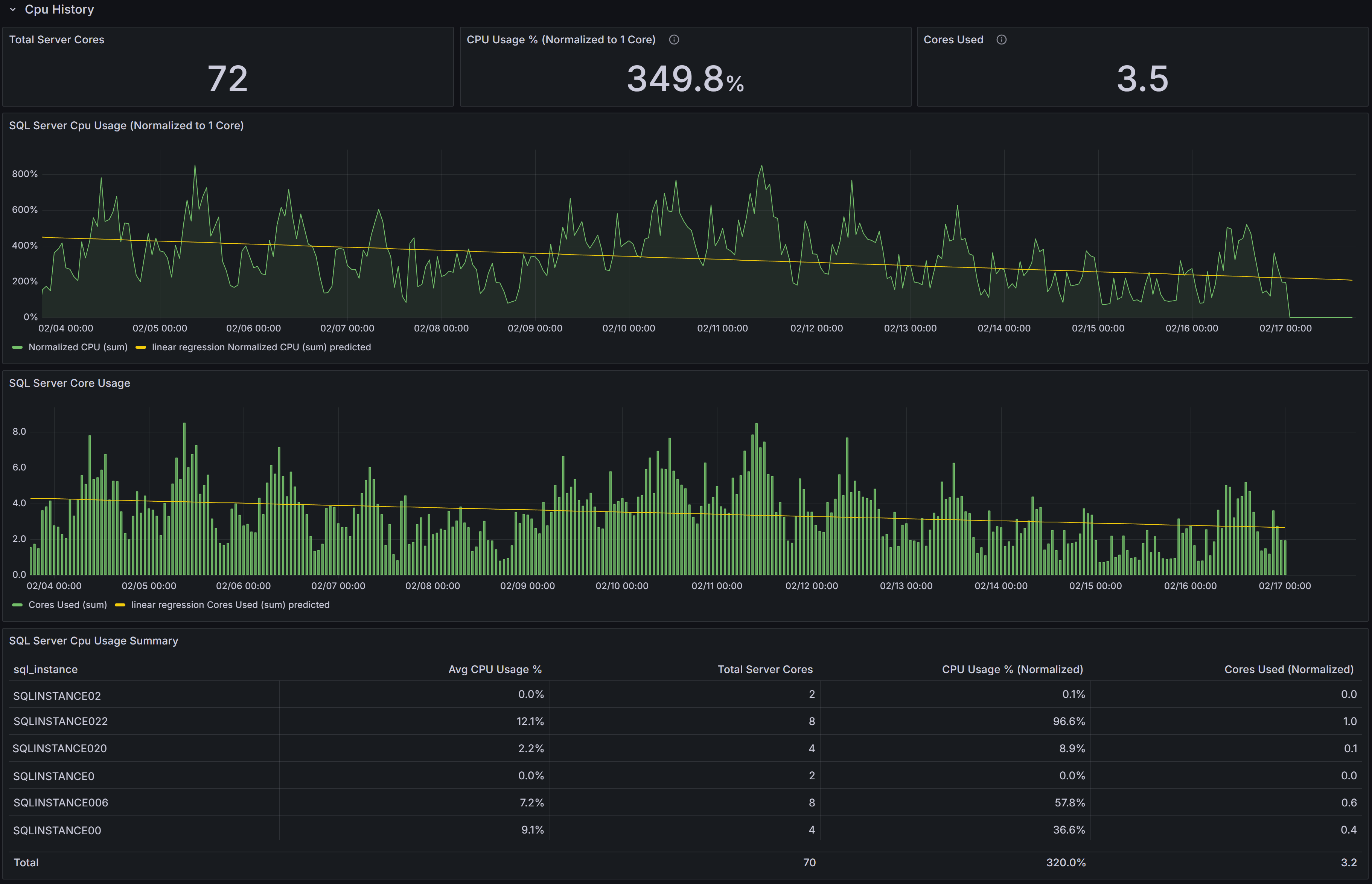Capacity Planning dashboard showing CPU trends

CPU KPIs

At the top of the section, three key performance indicators summarize CPU metrics across the selected instances:

Total Server Cores displays the aggregate number of CPU cores available across all selected instances. This gives you a sense of your total CPU capacity and helps with capacity planning calculations.

CPU Usage % (Normalized to 1 Core) expresses average CPU utilization on a per-core basis, normalized to a single-core equivalent. This normalization allows you to compare CPU intensity across servers with different core counts on equal footing.

Cores Used converts the normalized CPU percentage into an estimated count of cores actively in use across all selected instances. This is calculated as (Average CPU% × Total Server Cores ÷ 100). This metric provides an intuitive understanding of absolute CPU demand—if you see 3.1 cores used out of 24 total cores, you immediately understand both utilization intensity and available headroom.

CPU Usage Charts

Below the KPIs, two charts visualize CPU consumption patterns:

SQL Server CPU Usage (Normalized to 1 Core) shows each instance’s CPU utilization scaled to a single-core equivalent over time. This chart allows you to compare CPU intensity across instances with different core counts and identify which instances are experiencing the highest per-core pressure. Rising trends in this chart indicate increasing CPU usage that may eventually require optimization or additional capacity.

SQL Server Core Usage displays the estimated number of cores in use over time for each instance. This chart helps you understand aggregate core demand and evaluate capacity headroom. Sustained increases in this chart indicate growing workload that may eventually exhaust available capacity.

CPU Summary Table

The SQL Server CPU Usage Summary table ties the charts to individual instances and provides detailed per-instance metrics:

• SQL Instance identifies each server.
• Avg CPU Usage % shows the average CPU utilization over the selected time interval.
• Total Server Cores displays the number of CPU cores available on each host.
• CPU Usage % (Normalized) is calculated as Avg CPU% × Total Server Cores, showing the equivalent single-core utilization.
• Cores Used (Normalized) is calculated as (Avg CPU% × Total Server Cores) ÷ 100, showing the estimated number of cores actively utilized.

Use this table to rank instances by absolute CPU consumption and identify servers that would benefit from deeper investigation, query optimization, or workload redistribution. Sort by Cores Used to find instances with the highest absolute demand, or by CPU Usage % (Normalized) to find instances with the highest per-core intensity.

Interpreting CPU Trends

Look for rising trends in normalized CPU percentage or sustained high cores-used values. These patterns indicate growing CPU pressure that should be addressed before performance degrades. Sudden spikes may be acceptable if they correlate with known batch processes, but consistent baseline increases suggest permanent workload growth requiring capacity planning attention.

For instances with sustained high per-core utilization (above 70-80% normalized), these are candidates for:

• CPU capacity increases (more cores or larger VM SKUs)
• Workload redistribution to underutilized instances
• Deeper investigation using the Instance Overview dashboard to determine if optimization opportunities exist

Correlate CPU trends with memory, I/O, and wait-type metrics from other dashboards to form a complete capacity plan. CPU pressure combined with memory pressure may indicate that adding memory could reduce CPU load by improving cache hit ratios. CPU pressure combined with high CXPACKET waits may indicate parallelism tuning opportunities rather than capacity issues. Always allow headroom (commonly 20-30%) for growth and transient spikes unless autoscaling is available.

Data & Log Size

The Data & Log Size section tracks historical database file growth, helping you identify rapidly growing databases and plan storage capacity or maintenance before running out of disk space.

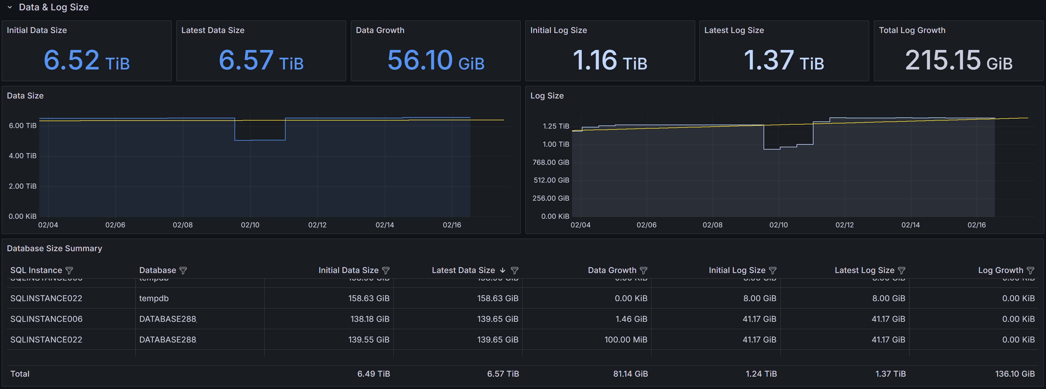Capacity Planning dashboard showing disk space usage trends

Storage KPIs

Six KPIs summarize data and log file growth across the selected instances:

Initial Data Size shows the total database data file size at the start of the selected time interval, typically displayed in terabytes or gigabytes. This establishes the baseline for measuring growth.

Latest Data Size displays the most recent total data file size, showing the current storage consumption.

Data Growth shows the increase in data file size between the initial and latest measurements, indicating how much storage has been consumed during the interval.

Initial Log Size shows the total transaction log file size at the start of the interval.

Latest Log Size displays the most recent total log file size.

Log Growth shows the change in log file size during the interval, which in well-maintained systems should be relatively stable or modest. Large log growth may indicate infrequent log backups, long-running transactions, or heavy bulk operations.

Storage Growth Charts

Two time-series charts visualize file size trends:

Data Size shows data file size changes over time for selected instances. Use this chart to detect steady linear growth indicating consistent workload increases, sudden jumps suggesting bulk data loads or new features, or unexpected decreases that may indicate data deletion or archiving activities.

Log Size shows transaction log file size trends over time. Log files in full recovery model grow until log backups truncate the inactive portion. Steadily growing log files often indicate infrequent log backups, while spikes may indicate large transactions or bulk operations. Consistently large logs may indicate long-running transactions preventing log truncation.

Database Size Summary Table

The Database Size Summary table provides per-database detail:

• SQL Instance and Database identify each database.
• Initial Data Size and Latest Data Size show data file sizes at the start and end of the interval.
• Data Growth shows the change in data file size.
• Initial Log Size and Latest Log Size show log file sizes at the start and end of the interval.
• Log Growth shows the change in log file size.

Use this table to rank databases by growth rate and identify candidates for archiving, compression, index maintenance, or retention policy changes. Sort by Data Growth to find the fastest-growing databases that may require additional storage allocation or investigation into why growth is occurring. Databases with large or growing log files deserve attention—investigate transaction patterns, backup frequency, and whether full recovery model is necessary for each database.

Interpreting Storage Trends

Rapid, sustained data growth may indicate new workloads, retention policy changes, missing cleanup jobs, or data hoarding without archiving strategies. Investigate recent application deployments, ETL process changes, or business requirement changes that might explain growth patterns. Compare growth rates with business metrics to determine whether growth is proportional to expected usage increases.

Large or growing log files often point to long-running transactions that prevent log truncation, infrequent log backups in full recovery mode, or heavy bulk operations. Review backup schedules to ensure log backups occur frequently enough (typically every 15-60 minutes for production databases). Investigate whether simple recovery model would be appropriate for databases that don’t require point-in-time recovery.

Use the time-range selector to analyze growth over different periods. Daily growth patterns help with immediate capacity planning, while weekly or monthly views reveal longer-term trends for strategic planning.

Disk Usage

The Disk Usage section shows historical disk I/O latency and throughput metrics, helping you identify storage performance bottlenecks and capacity issues that affect database performance.

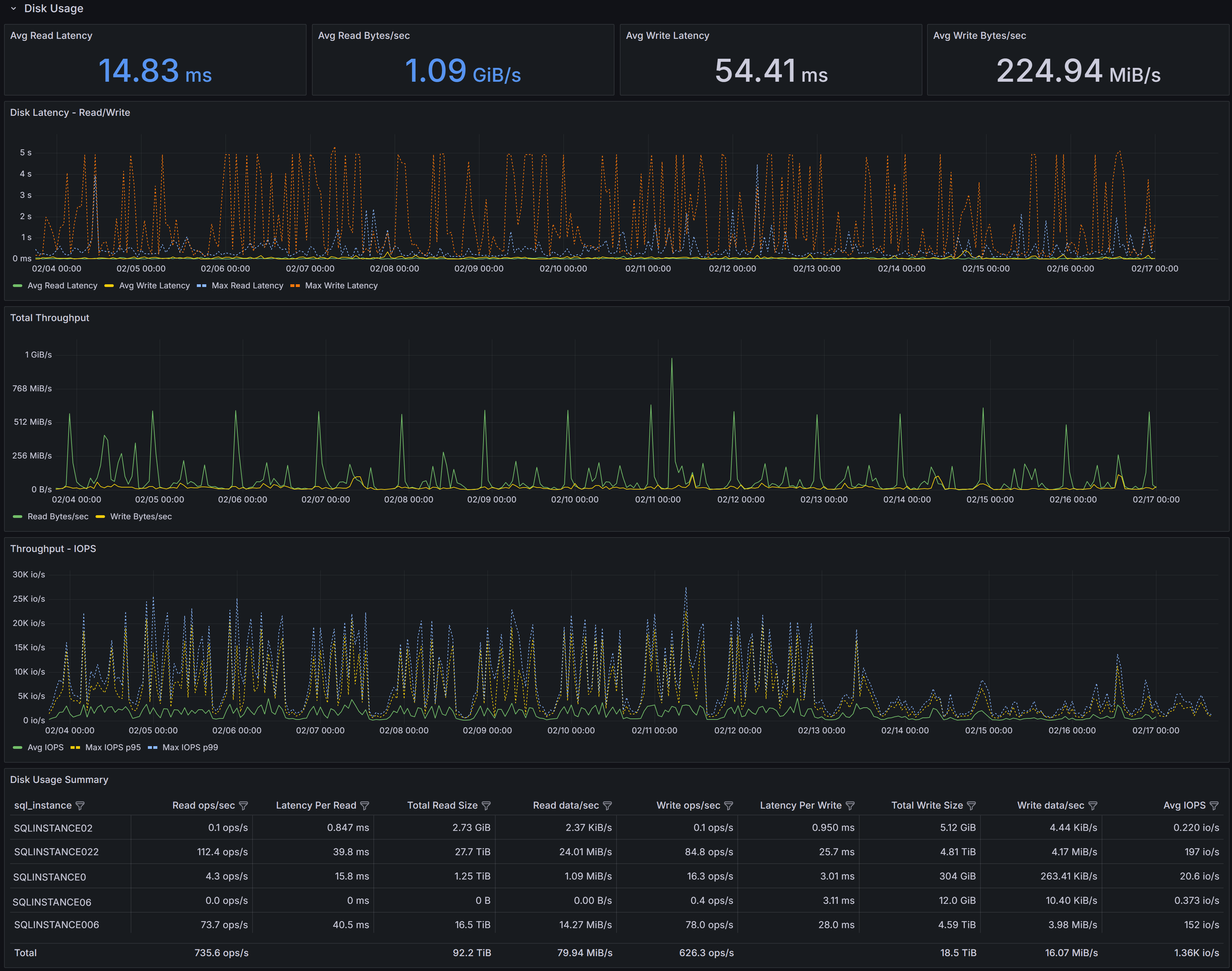Capacity Planning dashboard showing disk usage trends

Disk Performance KPIs

Four KPIs summarize I/O performance across selected instances:

Avg Read Latency shows the average time in milliseconds for read operations to complete during the selected interval. For modern SSD storage, read latency should typically be under 5ms. Values above 10-15ms may indicate storage performance issues, excessive concurrent load, or storage configuration problems.

Avg Read Bytes/sec displays average read throughput, showing how much data is being read from storage per second. This metric helps you understand whether storage bandwidth is being consumed and whether you’re approaching storage subsystem limits.

Avg Write Latency shows the average time in milliseconds for write operations to complete.

Avg Write Bytes/sec displays average write throughput, indicating how much data is being written to storage per second.

I/O Performance Charts

Three time-series charts visualize I/O patterns over the selected time range:

Disk Latency - Reads/Write shows both average read latency and average write latency plotted together over time, along with maximum read and write latency values. The chart displays four series: Avg Read Latency, Avg Write Latency, Max Read Latency, and Max Write Latency. Use this chart to spot periods of elevated latency and correlate them with workload changes, concurrent activity, or storage system issues. Consistent high latency indicates chronic storage performance problems, while intermittent spikes may correlate with specific queries, batch jobs, or checkpoint activity. Pay particular attention to the gap between average and maximum latency—large gaps indicate inconsistent storage performance that may cause unpredictable application response times.

Total Throughput displays both read and write throughput (in bytes per second) on the same chart, allowing you to see the overall I/O bandwidth consumption pattern. Sustained high read throughput may indicate memory pressure forcing more physical reads, queries performing large scans, or increased workload. Regular spikes in write throughput for data files typically correspond to checkpoint intervals, while consistent write throughput reflects transaction activity levels. Compare read and write patterns to understand whether your workload is read-heavy, write-heavy, or balanced.

Throughput - IOPS shows I/O operations per second for reads and writes, along with maximum IOPS values. This chart displays Avg IOPS, Max IOPS (read), and Max IOPS (write).

Spikes in IOPS often correlate with index maintenance operations, checkpoint activity, or queries performing many small reads.

Disk Usage Summary Table

The Disk Usage Summary table provides detailed per-instance I/O metrics:

• SQL Server Instance identifies each server.
• Read ops/sec shows the average number of read operations per second, indicating read workload intensity.
• Latency Per Read displays average read latency in milliseconds for each instance.
• Total Read Size shows the cumulative amount of data read during the interval.
• Read data/sec displays read throughput rate.
• Write ops/sec shows the average number of write operations per second.
• Latency Per Write displays average write latency in milliseconds for each instance.
• Total Write Size shows the cumulative amount of data written during the interval.
• Write data/sec displays write throughput rate.
• Avg IOPS shows the average I/O operations per second (combined read and write) for each instance.

Use this table to rank instances by I/O pressure and prioritize investigation or remediation. Instances with high latency deserve immediate attention, especially if write latency is high on instances with transaction-heavy workloads. Sort by Latency Per Write to identify instances where transaction performance may be impacted by slow log writes. Sort by IOPS to find instances with the most I/O-intensive workloads that may be approaching storage system limits.

Interpreting I/O Metrics

Elevated read or write latency often points to storage contention, slow disk subsystems, high queue depth, or insufficient storage IOPS capacity. Correlate latency with throughput and IOPS metrics—high throughput with acceptable latency suggests the storage system is handling load well, while high latency with moderate throughput indicates the storage system is struggling.

High read throughput with low latency may indicate healthy buffer cache behavior and good storage performance. High read throughput with rising latency suggests memory pressure forcing excessive physical reads that the storage system cannot efficiently handle. In this case, adding memory may be more effective than upgrading storage.

For write-heavy workloads with high latency, review transaction patterns and log file placement. Ensure transaction log files are on fast storage separate from data files. Consider faster storage tiers (NVMe SSDs), enabling write caching with proper battery backup, or reviewing checkpoint interval settings to spread write load more evenly.

High IOPS with relatively low throughput typically indicates many small random I/O operations, which are more demanding on storage systems than sequential operations. This pattern is common in OLTP workloads and may benefit from faster storage (SSDs instead of HDDs) or better indexing to reduce the number of I/O operations required per query.

Large gaps between average and maximum latency or IOPS indicate inconsistent storage performance. This can cause unpredictable application response times even when average metrics look acceptable. Investigate whether storage system resource contention, competing workloads, or storage controller issues are causing the variability.

Use the time-range selector to isolate problematic time windows and correlate with Query Stats, CPU, and other dashboards before making hardware changes or storage tier upgrades. Sometimes what appears to be storage problems are actually caused by inefficient queries that can be optimized, eliminating the need for storage investments.

Memory Usage

The Memory Usage section shows memory allocation and demand patterns, helping you detect memory pressure and plan memory changes or workload placement decisions.

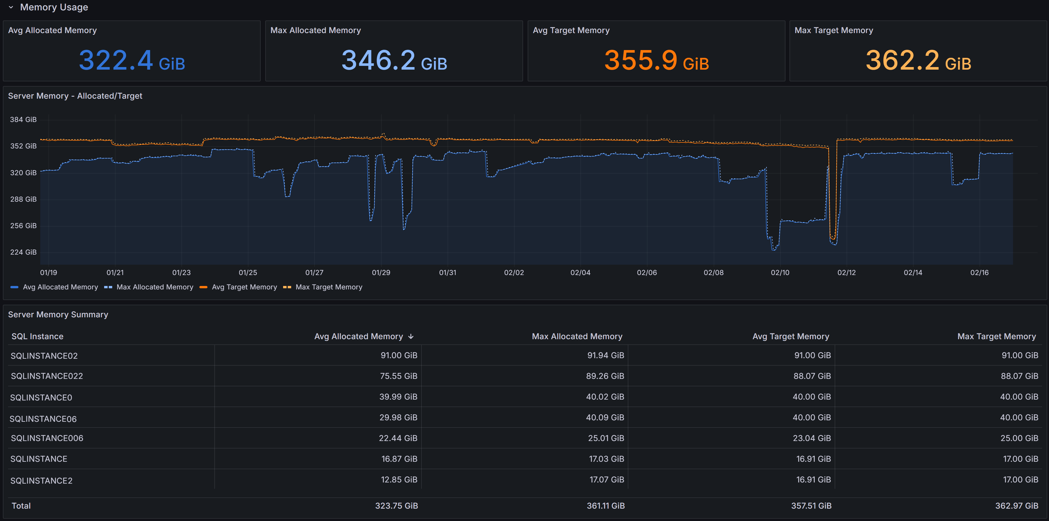Capacity Planning dashboard showing memory trends

Memory KPIs

Four KPIs summarize memory metrics:

Server Memory - Allocated/Target displays both current allocated memory and target memory.

Max Allocated Memory shows the peak memory allocation observed during the selected interval

Avg Target Memory displays the average target memory SQL Server attempted to obtain based on workload demand and configuration. When target memory exceeds allocated memory consistently, SQL Server is experiencing memory pressure and would benefit from additional memory.

Max Target Memory shows the peak target memory during the interval

Memory Usage Charts

The Server Memory - Allocated/Target chart shows memory allocation and target over time for each instance. Use this chart to spot sustained allocation near target (indicating memory pressure) or gaps between allocated and target that may indicate memory configuration limits, OS constraints, or other factors preventing SQL Server from obtaining desired memory.

Server Memory Summary Table

The table provides per-instance memory metrics:

• SQL Instance identifies each server.
• Avg Allocated Memory shows average memory allocation during the interval.
• Max Allocated Memory displays peak allocation.
• Avg Target Memory shows average memory target.
• Max Target Memory displays peak target.

Use this table to rank instances by memory consumption and identify candidates for memory increases, VM resizing, or workload redistribution.

Interpreting Memory Metrics

When allocated memory consistently tracks close to target memory, SQL Server is successfully obtaining the memory it needs. Large gaps between target and allocated memory may indicate:

• Max server memory configuration set too low
• OS memory pressure limiting SQL Server allocation
• locked pages configuration issues
• Memory grants waiting or unable to be satisfied

Correlate memory trends with I/O metrics from the Disk Usage section. If memory pressure coincides with high read latency and read throughput, adding memory will likely reduce I/O load by improving buffer cache hit ratios, potentially providing better performance improvement than storage upgrades.

Review Page Life Expectancy and Memory Grants Pending in the Instance Overview dashboard alongside capacity planning memory data. When memory pressure is evident, this strongly indicates that additional memory will improve performance by reducing physical reads and improving query execution efficiency.

Using the Dashboard Effectively

Time Ranges: Use shorter ranges (days) for immediate issues, longer ranges (weeks/months) for trend analysis and capacity planning.

Correlation is Key: Combine capacity planning with Query Stats, Instance Overview, and I/O Analysis dashboards. High CPU with expensive queries suggests optimization before adding capacity. High I/O with memory pressure suggests adding memory before upgrading storage.

Plan with Headroom: Maintain 20-30% available capacity for growth and spikes unless autoscaling is available. Size for peak utilization, not just averages.

Regular Review: Revisit capacity metrics monthly or quarterly. Document baselines to track trends and adjust plans as workloads evolve.

1.7 - SQL Server Agent Jobs

The SQL Server Agent Jobs dashboard provides comprehensive visibility into job execution history and current job status across your SQL Server instances. This dashboard helps you monitor job health, identify failures, investigate scheduling conflicts, and analyze job duration patterns to ensure critical maintenance tasks, ETL processes, and scheduled operations complete successfully and on time.

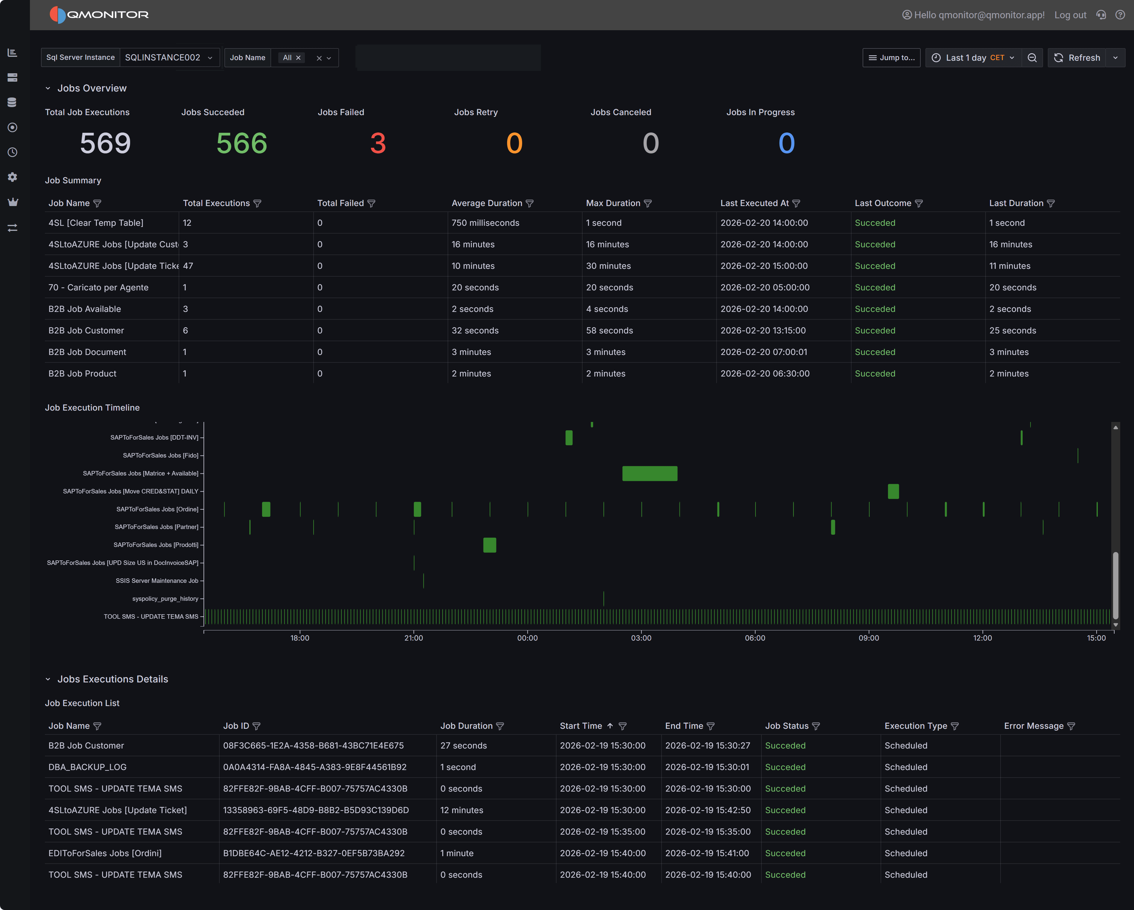SQL Server Agent Jobs dashboard showing job executions, timeline, and detailed history

The SQL Server Agent Jobs dashboard provides a compact view of job activity and execution history so you can monitor health, spot failures, and investigate scheduling or duration issues.

Dashboard Sections

Jobs Overview

The Jobs Overview section provides high-level KPIs that summarize job execution activity across the selected time interval and instances:

• Total Job Executions shows the total number of job runs observed during the selected period, giving you a sense of overall job activity and scheduling density.

• Jobs Succeeded displays the count of jobs that completed successfully without errors.

• Jobs Failed shows the number of jobs that finished with errors.

• Jobs Retried displays runs that were automatically retried after transient failures. High retry counts may indicate intermittent issues like blocking, timeouts, or resource contention that should be investigated.

• Jobs Canceled shows jobs that were manually canceled or programmatically terminated before completion.

• Jobs In Progress displays currently running jobs.

Use these KPIs for a quick health check and to detect elevated failure or retry rates that need attention. Compare current metrics with historical baselines to identify degrading trends.

Job Summary

The Job Summary table groups executions by job name and provides aggregate statistics for each job during the selected time interval:

• Job Name identifies each SQL Server Agent job.
• Total Executions shows how many times the job ran during the interval.
• Average Duration displays the typical execution time, useful for detecting anomalies.
• Max Duration shows the longest execution time.
• Last Executed At displays when the job last ran.
• Last Outcome shows whether the most recent execution succeeded or failed.
• Last Duration displays how long the most recent execution took.

Sort by Total Failed to find jobs with the highest failure rates that need immediate attention. Sort by Max Duration to identify jobs experiencing performance issues or unexpected delays. Filter by job name or outcome to focus on specific jobs or failure scenarios.

Job Execution Timeline

The Job Execution Timeline provides a visual Gantt-style representation of job executions over time, with each job displayed as a separate row and individual executions shown as horizontal bars.

Execution bars are color-coded by status:

• Green indicates successful completion
• Red indicates failure
• Blue or other colors may indicate in-progress or retry states

This timeline visualization is particularly valuable for:

Identifying Scheduling Conflicts: Overlapping bars for different jobs indicate concurrent execution, which may cause resource contention, blocking, or performance degradation. If critical jobs consistently overlap, consider staggering their schedules.

Finding the appropriate time window to schedule new jobs: Look for gaps in the timeline where no jobs are running to identify optimal time windows for scheduling new jobs, especially those that are resource-intensive.

Spotting Duration Patterns: Wide bars indicate long-running executions. If a job’s execution bars are consistently wider than historical patterns, investigate whether data volume increases, performance degradation, or blocking are causing delays.

Detecting Failure Clusters: Multiple red bars at the same time across different jobs may indicate infrastructure-wide issues like server resource exhaustion, storage problems, or maintenance windows affecting multiple processes.

Understanding Job Frequency: The spacing between bars for the same job shows its execution frequency. Jobs that run too frequently may need schedule optimization, while jobs with large gaps may indicate scheduling problems or dependencies preventing execution.

Use the timeline’s zoom and pan controls to focus on specific time windows and correlate job activity with other performance metrics from Instance Overview or Query Stats dashboards.

Job Execution Details

The Job Execution Details table lists every individual job execution during the selected time interval with complete context:

• Job Name identifies which job ran.
• Job ID provides the unique SQL Server Agent job identifier (GUID).
• Job Duration shows how long the execution took to complete.
• Start Time displays when the execution began.
• End Time shows when the execution completed (or when it was canceled/failed).
• Job Status indicates the outcome: Succeeded, Failed, Canceled, or In Progress.
• Execution Type shows how the job was initiated: Scheduled (by SQL Server Agent scheduler), Manual (started by a user or another process), or other triggers.
• Error Message displays the error text when jobs fail, providing immediate diagnostic information.

Sort by Job Duration to find the longest-running executions that may indicate performance problems. Filter by Job Status = Failed to focus on troubleshooting failures. Use Start Time sorting to understand chronological execution order and identify when specific issues occurred.

Investigation tips

• Filter by instance, owner, or outcome to isolate problematic jobs.
• Correlate job failures and long durations with CPU, I/O, and blocking at the same timestamps to find root causes.
• For recurring transient failures, consider retry logic or schedule changes to avoid resource contention windows.
• Use the timeline to detect overlapping schedules; stagger long-running jobs to reduce contention.

Investigating Job Issues

When analyzing job execution problems, use these strategies to identify root causes:

Correlate with System Metrics: Job failures and long durations often correlate with system-wide issues. Use the Instance Overview dashboard to check whether CPU pressure, memory constraints, or I/O bottlenecks occurred during problematic job executions. Review the Blocking and Deadlocks dashboards to determine whether locking issues delayed or failed jobs.

Analyze Failure Patterns: Look for patterns in job failures�do they occur at the same time of day, on specific days of the week, or in conjunction with other jobs? Failures clustered around maintenance windows, backup times, or batch processing periods may indicate resource contention or inadequate time windows.

Investigate Duration Increases: Jobs that gradually take longer to execute may indicate data growth, index fragmentation, outdated statistics, or missing indexes. Compare current durations with historical averages to detect performance degradation. Jobs that suddenly take much longer may indicate blocking, resource exhaustion, or query plan changes.

Review Retry Patterns: High retry counts suggest intermittent issues like transient blocking, timeouts, or network problems. Review job step retry logic to ensure it’s appropriate�some failures like logic errors won’t be resolved by retries, while others like deadlocks may succeed on retry. Consider implementing exponential backoff for retry delays.

Detect Scheduling Conflicts: Use the timeline to identify overlapping jobs that may compete for resources. Stagger long-running maintenance jobs, index rebuilds, and backup operations to reduce contention. Consider using job dependencies and precedence constraints to serialize jobs that should not run concurrently.

Monitor Resource-Intensive Jobs: Jobs that consistently consume high CPU, generate excessive I/O, or hold locks for extended periods may impact other workloads. Review job step queries using the Query Stats dashboard to identify optimization opportunities.

1.8 - Index Analysis

The Index Analysis dashboard helps you prioritize index optimization work by identifying high-value missing index opportunities and surfacing existing indexes that may be hurting performance. This dashboard analyzes index usage patterns to guide decisions about which indexes to create, which to remove, and which to consolidate, helping you balance query performance improvements against the costs of index maintenance and storage.

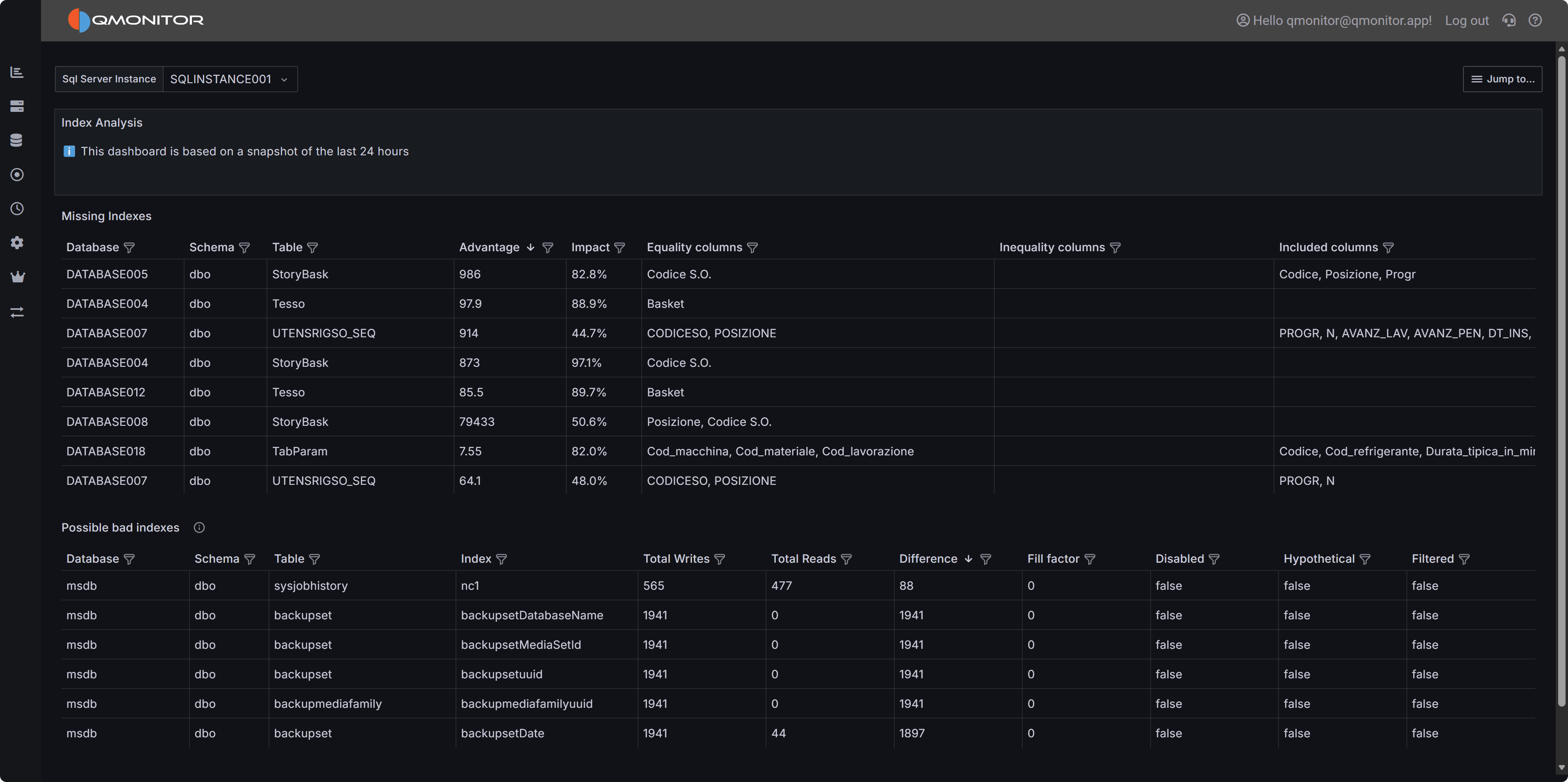Index Analysis dashboard showing missing index recommendations and underutilized existing indexes

Dashboard Sections

Missing Indexes

The Missing Indexes section displays optimizer-suggested indexes that could improve query performance. SQL Server’s query optimizer tracks situations where an index would have been beneficial during query execution, and this dashboard surfaces those recommendations prioritized by potential impact.

The table includes the following columns to help you evaluate each missing index suggestion:

• Database identifies which database would benefit from the index.
• Schema shows the schema name containing the table.
• Table displays the table name that needs the index.
• Advantage provides an estimate of the expected improvement, typically measured in reduced logical reads or improved query execution time.
• Impact shows a percentage representing the relative benefit of this index across the entire workload. Higher impact values indicate indexes that would benefit more queries or more frequently-executed queries.
• Equality columns lists columns recommended for equality predicates (WHERE column = value). These become the key columns of the index and should appear first in the index definition.
• Inequality columns lists columns recommended for range predicates (WHERE column > value, BETWEEN, etc.). These should appear after equality columns in the key.
• Included columns lists non-key columns suggested for covering queries. Including these columns allows queries to satisfy all their column needs from the index without looking up data in the base table.

Sort by Impact to find the highest-value missing indexes that would benefit the most queries. Sort by Advantage to identify indexes that would provide the greatest improvement to individual query performance. Filter by Database or Table to focus optimization efforts on specific areas.

Evaluating Missing Index Recommendations

When considering whether to create a suggested index:

Assess the Impact: High-impact suggestions (above 80%) typically represent significant optimization opportunities affecting many queries or critical workloads. Lower-impact suggestions may not justify the overhead.

Review the Column Lists: Equality columns, inequality columns, and included columns together define the complete index structure. Ensure the suggested column order makes sense for your queries. Sometimes reordering columns or creating multiple smaller indexes is more effective than the exact suggested structure.

Consider Write Overhead: Every index must be maintained during INSERT, UPDATE, and DELETE operations. Tables with heavy write workloads may not benefit from additional indexes despite optimizer suggestions. Balance read performance improvements against write performance costs.

Check for Overlapping Indexes: Before creating a new index, review existing indexes on the same table. You may be able to modify an existing index to cover the missing index scenario rather than creating an entirely new index. Consolidating indexes reduces storage and maintenance overhead.

Validate with Actual Queries: Identify the specific queries that would benefit from the suggested index using the Query Stats dashboard. Test those queries with the proposed index to verify the performance improvement matches expectations. Sometimes query optimization or statistics updates are more effective than adding indexes.

Evaluate Storage Impact: Large indexes on large tables consume significant storage and memory. Ensure you have capacity for the new index and that it won’t negatively impact buffer pool efficiency by consuming memory needed for data pages.

Possible Bad Indexes

The Possible Bad Indexes section identifies existing indexes that may be candidates for removal or consolidation because they incur maintenance overhead without providing sufficient query performance benefits. These indexes consume storage, slow down write operations, and use buffer pool memory that could be better utilized elsewhere.

The table displays the following information:

• Database shows which database contains the index.
• Schema displays the schema name.
• Table shows the table containing the index.
• Index displays the index name.
• Total Writes shows the cumulative number of write operations (inserts, updates, deletes) that affected this index during the analysis period. High write counts indicate significant maintenance overhead.
• Total Reads displays the cumulative number of read operations (seeks, scans, lookups) that used this index. Low read counts suggest the index isn’t providing much query benefit.
• Difference shows Total Writes minus Total Reads. Large positive values indicate write-heavy indexes with minimal read usage—strong candidates for removal.
• Fill factor displays the configured fill factor percentage. Lower values (like 70-80%) leave space for inserts but consume more storage and may indicate fragmentation concerns.
• Disabled indicates whether the index is currently disabled. Disabled indexes still consume storage but aren’t used by queries—they should generally be removed unless temporarily disabled for maintenance.
• Hypothetical shows whether the index is hypothetical (created with STATISTICS_ONLY). Hypothetical indexes are usually remnants of tools like Database Engine Tuning Advisor and should be removed if not
• actively used for testing.
• Filtered indicates whether the index uses a filter predicate (WHERE clause). Filtered indexes apply to a subset of rows and may have different usage patterns than full-table indexes.

Sort by Difference to find indexes with the highest write-to-read ratio. Filter by Disabled = true to find indexes that should be removed immediately. Filter by Total Reads = 0 to find completely unused indexes.

Investigating Underutilized Indexes

When evaluating whether to remove or consolidate an index:

Analyze Usage Patterns Over Time: The dashboard shows 24-hour activity, but some indexes support monthly reporting, quarterly processes, or annual operations. Analyze index usage over longer periods before dropping indexes that appear unused.

Check for Foreign Key Relationships: Indexes supporting foreign key constraints are often critical for delete operations and join performance even if they show low read counts. Verify whether the index supports a foreign key before considering removal.

Review Unique and Primary Key Constraints: Indexes enforcing uniqueness or primary key constraints cannot be dropped without removing the constraint. These indexes serve data integrity purposes beyond query optimization.

Consider Index Consolidation: Instead of dropping an index entirely, consider whether it could be modified or merged with another index to reduce the total index count while preserving query performance. For example, an index on (Column1, Column2) can often replace separate indexes on (Column1) and (Column2).

Evaluate Filtered Index Opportunities: Write-heavy indexes with low read counts might be better implemented as filtered indexes covering only the rows frequently queried. This reduces write overhead while maintaining query performance for the important subset of data.

Test in Non-Production: Create a test environment, drop the candidate index, and run representative workloads. Monitor query performance and execution plans to verify no queries are negatively impacted. Pay special attention to batch processes, reports, and administrative operations.

Using the Dashboard Effectively

Regular Review: Analyze index recommendations monthly or quarterly to identify new optimization opportunities as workloads evolve. Index needs change over time as data volumes grow and query patterns shift.

Prioritize High-Impact Work: Focus first on missing indexes with impact above 80% and existing indexes with Difference (writes - reads) above 10,000. These represent the clearest optimization opportunities with the most significant potential benefit.

Balance Read and Write Performance: Creating indexes improves read performance but degrades write performance. For write-heavy tables, be more conservative about adding indexes. For read-heavy tables, missing index recommendations are more likely to provide net benefit.

Cross-Reference with Query Stats: Use the Query Stats dashboard to identify which specific queries would benefit from suggested indexes or are affected by index removal. This provides concrete data to validate index decisions rather than relying solely on estimates.

Document Decisions: When creating or dropping indexes based on this dashboard, document the reasoning, expected impact, and actual results. This helps track whether index changes deliver expected benefits and guides future optimization work.

Consider Maintenance Windows: Creating large indexes can be resource-intensive and may impact production workloads. Schedule index creation during maintenance windows using the ONLINE option where available to minimize disruption.

1.9 - Always On Availability Groups

The Always On Availability Groups dashboard provides comprehensive visibility into the health and status of SQL Server Always On Availability Groups across your monitored instances. This dashboard helps you quickly verify AG configuration, monitor replica synchronization status, identify failover readiness issues, and ensure your high availability infrastructure is operating correctly.

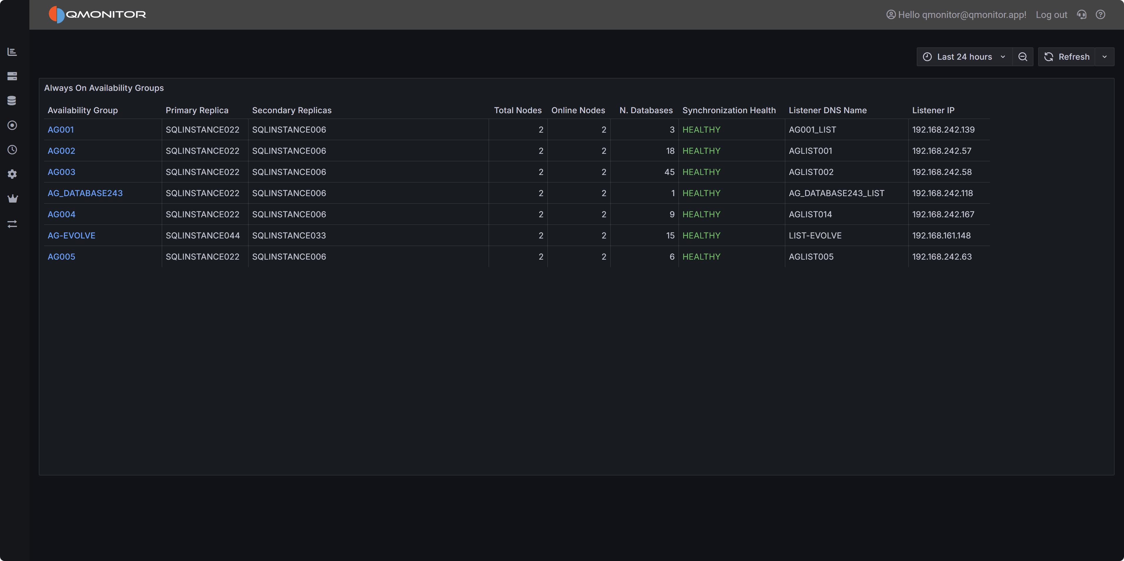Always On Availability Groups dashboard showing AG health, replica status, and synchronization state

Dashboard Overview

The dashboard displays a summary table of all configured Availability Groups across your SQL Server estate, making it easy to assess the health of your high availability infrastructure at a glance. Use this dashboard to perform regular health checks, verify failover readiness, and quickly identify AGs requiring investigation or intervention.

Availability Groups Table

The Availability Groups table provides detailed information about each configured AG:

Availability Group displays the AG name as a clickable link. Click the AG name to open the detailed AG dashboard showing per-replica metrics, database synchronization progress, redo queue depth, and comprehensive failover readiness information.

Primary Replica shows the current primary replica hostname. The primary replica handles all read-write operations and is the source for transaction log records sent to secondary replicas. In a properly functioning AG, this should match your expected primary server. If the primary is unexpected, a failover may have occurred that requires investigation.

Secondary Replicas displays a comma-separated list of all configured secondary replica hostnames. Secondary replicas receive transaction log records from the primary and can serve read-only workloads depending on configuration. This column helps you quickly verify all expected replicas are configured.

Total Nodes shows the total number of replicas configured in the AG, including the primary. Most AGs have 2-3 replicas, though SQL Server supports more for specific scenarios. This count should match your expected AG topology.

Online Nodes displays how many replicas are currently online and reachable. This should equal Total Nodes in a healthy AG. Values less than Total Nodes indicate one or more replicas are offline, disconnected, or experiencing connectivity issues, a critical situation requiring immediate investigation.

N. Databases shows the number of databases protected by this AG. This helps you understand the scope and importance of each AG. AGs protecting many databases or critical systems deserve closer monitoring.

Synchronization Health displays the overall synchronization state of the AG, typically showing “HEALTHY” (in green) when all replicas are synchronized and failover-ready, or “NOT HEALTHY” when synchronization issues exist. Unhealthy synchronization states indicate data protection risks and potential failover problems.

Listener DNS Name shows the AG listener’s DNS name if configured. Applications should connect to this listener name rather than directly to instance names, allowing transparent failover without connection string changes.

Listener IP displays the IP address or addresses associated with the AG listener. In multi-subnet configurations, multiple IPs may appear. Verify these IPs match your expected listener configuration.

Using the Dashboard

Regular Health Checks: Review this dashboard daily to verify all AGs show “HEALTHY” synchronization status and all configured replicas are online. Early detection of synchronization issues prevents data loss during failovers.

Drill Down for Details: Click any AG name to access the detailed AG dashboard showing replica-level metrics including synchronization state, redo queue depth, log send rate, and database-specific synchronization status. Use these details to diagnose synchronization delays or performance issues.

Verify After Failovers: After planned or unplanned failovers, use this dashboard to confirm the expected server is now primary and all replicas have resynchronized. Verify listener DNS and IP addresses resolve correctly to the new primary.

Monitor Synchronization Health: “NOT HEALTHY” status requires immediate investigation. Common causes include network issues, replica performance problems, long-running transactions on the primary, or redo thread bottlenecks on secondaries. The detailed AG dashboard provides metrics to pinpoint the root cause.

Track Replica Topology: Use the Total Nodes and Secondary Replicas columns to maintain awareness of your AG configuration. Changes to expected topology may indicate configuration drift or unauthorized modifications requiring investigation.

Investigating Issues

Offline Replicas: When Online Nodes is less than Total Nodes, check whether the offline replica is stopped, whether Windows Server Failover Clustering (WSFC) quorum is healthy, whether network connectivity exists between replicas, or whether the SQL Server service is running on the offline node.

Unhealthy Synchronization: Synchronization health issues may result from network bandwidth limitations preventing log records from reaching secondaries quickly enough, secondary replica performance problems causing redo queue buildup, transaction log I/O bottlenecks on primary or secondary replicas, or very large transactions overwhelming synchronization capacity.

Unexpected Primary Replica: If the primary replica is not the expected server, determine whether a planned failover occurred, whether an automatic failover responded to a failure, whether a manual failover was performed without proper communication, or whether cluster node preferences have changed.

Missing or Incorrect Listener Information: Verify the listener is properly configured in Windows Server Failover Clustering, confirm DNS records exist and resolve correctly, check that listener IP addresses are reachable from application servers, and ensure no firewall rules block listener ports.

Related Dashboards

Use the Instance Overview dashboard to check resource utilization, performance metrics, and wait statistics on primary and secondary replicas. High CPU, memory pressure, or I/O bottlenecks can impact AG synchronization performance.

Review the Blocking and Deadlocks dashboards if synchronization issues correlate with locking problems. Long-running transactions holding locks can delay log truncation and impact AG performance.

Check the SQL Server I/O Analysis dashboard to evaluate transaction log write performance on both primary and secondary replicas. Slow log I/O directly impacts synchronization speed and data protection.

1.9.1 - Always On Availability Group Detail

The Always On Availability Group Detail dashboard provides comprehensive health and replication metrics for a single Availability Group, allowing you to monitor replica status, track failover history, analyze data movement performance, and identify synchronization issues. This dashboard is essential for troubleshooting AG problems, verifying failover readiness, and ensuring your high availability infrastructure operates optimally.

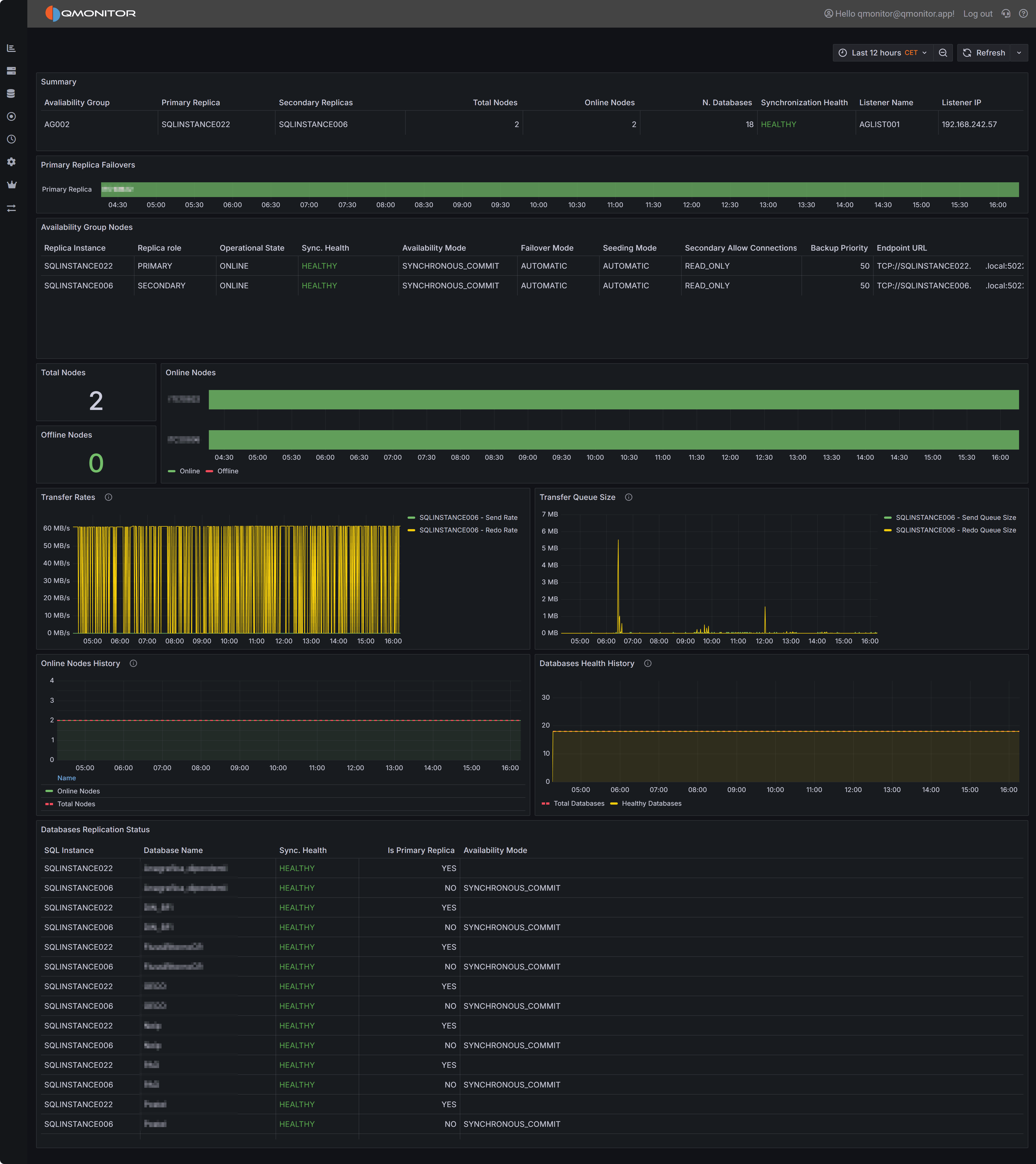Availability Group Detail dashboard showing replica health, failover history, and replication metrics

Dashboard Sections

AG Summary

The summary section at the top displays key information about the Availability Group configuration and current state:

Availability Group displays the AG name for reference.

Primary Replica shows the current primary replica hostname. This is the replica handling all read-write operations and serving as the transaction log source for secondary replicas.

Secondary Replicas lists all configured secondary replica hostnames, showing your AG topology at a glance.

Total Nodes displays the total number of replicas configured in the AG, including primary and all secondaries.

Online Nodes shows how many replicas are currently online and reachable. This should equal Total Nodes in a healthy AG. Lower values indicate offline replicas that reduce redundancy and may prevent automatic failover.

N. Databases shows the number of databases protected by this AG.

Synchronization Health displays the overall synchronization state, typically “HEALTHY” when all databases on all replicas are synchronized and ready for failover, or showing issues when synchronization problems exist.

Listener Name displays the AG listener’s DNS name if configured. Applications should connect via this listener for automatic failover support.

Listener IP shows the IP address or addresses associated with the listener.

Primary Replica Failovers

The Primary Replica Failovers timeline visualizes which replica was primary at each point during the selected time range. This horizontal timeline shows the primary role assignment over time, with color-coded bars indicating which server held the primary role during each period.

Use this timeline to review recent failover history and understand failover frequency and patterns. Frequent failovers may indicate instability, while unexpected failovers during business hours require investigation. Correlate failover times with events from the Instance Overview or Events dashboards to identify what triggered role changes—planned maintenance, automatic failover due to health detection, or manual intervention.

Availability Group Nodes

The Availability Group Nodes table provides detailed configuration and status information for each replica:

Replica Instance shows the SQL Server instance name for each replica in the AG.

Replica role indicates whether the replica is currently PRIMARY or SECONDARY. Only one replica is primary at any time.

Operational State shows the current operational status of each replica (ONLINE, OFFLINE, etc.).

Sync. Health displays the per-replica synchronization status. “HEALTHY” indicates the replica is properly synchronized with the primary. Unhealthy states indicate synchronization problems requiring investigation.

Availability Mode shows whether the replica uses SYNCHRONOUS_COMMIT (waits for secondary acknowledgment before committing transactions, ensuring zero data loss) or ASYNCHRONOUS_COMMIT (commits without waiting, better performance but potential data loss during failover).

Failover Mode indicates whether the replica supports AUTOMATIC failover (can automatically become primary if the current primary fails) or MANUAL failover (requires manual intervention to become primary).

Seeding Mode shows whether the replica uses AUTOMATIC seeding (SQL Server automatically copies database files to initialize the replica) or MANUAL seeding (database files must be manually restored).

Secondary Allow Connections displays the read-intent settings for secondary replicas: NO (no connections allowed), READ_ONLY (only read-only connections allowed), or ALL (all connections allowed).

Backup Priority shows the priority value used for backup preference routing. Higher values indicate preferred backup targets when using AG-aware backup strategies.

Endpoint URL displays the database mirroring endpoint URL used for data movement between replicas.

R/O Routing URL shows the read-only routing address if configured, used to direct read-only queries to secondary replicas.

R/W Routing URL displays the read-write routing address if configured.

Node Availability Metrics

The Node Availability section provides KPIs and visualization of replica online status:

Total Nodes KPI shows the configured replica count for quick reference.

Offline Nodes KPI displays how many replicas are currently offline. This should be 0 in a healthy AG.

Online Nodes chart plots the number of online replicas over time during the selected interval. A consistently flat line at the total node count indicates stable availability. Dips indicate periods when replicas went offline, while fluctuating lines suggest flapping replicas with intermittent connectivity issues.

Transfer Rates and Queue Sizes

These charts visualize data movement performance between primary and secondary replicas:

Transfer Rates chart displays:

• Send Rate: How fast the primary replica sends transaction log records to secondaries, measured in MB/s or KB/s. Higher values indicate more transaction activity requiring replication.
• Redo Rate: How fast secondary replicas apply received transaction log records to their databases. Redo rate should keep pace with send rate to maintain synchronization.

Low or decreasing redo rates on secondaries indicate performance bottlenecks. Common causes include slow storage I/O on secondaries, CPU pressure preventing redo threads from keeping up, or blocking on secondaries due to read workloads holding locks that conflict with redo operations.

Transfer Queue Size chart shows:

• Send Queue Size: Amount of transaction log data (in KB or MB) waiting on the primary to be sent to secondaries. Growing send queues indicate network bandwidth limitations or secondary connectivity issues.
• Redo Queue Size: Amount of transaction log data received by secondaries but not yet applied. Growing redo queues indicate secondaries cannot keep pace with transaction volume, creating synchronization lag that increases RPO (potential data loss during failover) and may delay failover readiness.

Health History

The health history section provides time-series visualization of AG health trends:

Online Nodes History chart plots total nodes versus online nodes over time, showing historical availability patterns. Consistent alignment between total and online nodes indicates stable replica availability. Gaps indicate periods with offline replicas.

Database Health History chart shows total databases in the AG versus healthy databases over time. When these lines separate, one or more databases have become unsynchronized or unhealthy, requiring investigation. This may result from synchronization issues, suspended data movement, or database-specific problems.

Databases Replication Status

The Databases Replication Status table provides per-database synchronization details across all replicas:

SQL Instance shows which replica hosts each database copy.

Database Name identifies the database.

Sync. Health displays the synchronization status for this database on this replica. “HEALTHY” indicates proper synchronization with the primary, while other states indicate issues.

Is Primary Replica shows whether this row represents the primary copy (YES) or a secondary copy (NO).

Availability Mode displays the availability mode for this database replica, typically inheriting from the AG-level configuration but potentially overridden per database in some configurations.

Use this table to identify which specific databases have synchronization problems when overall AG health shows issues. Sort by Sync. Health to find unhealthy databases requiring attention. Filter by specific databases to see their status across all replicas.

Investigating Synchronization Issues

Growing Redo Queues: When redo queue sizes increase steadily, investigate secondary replica performance. Check the Instance Overview dashboard for the secondary—look for high CPU utilization, memory pressure, or I/O bottlenecks. Review the SQL Server error log on secondaries for redo thread errors or warnings. Consider whether read workloads on secondaries are causing blocking that interferes with redo operations.

Low Redo Rates: Consistently low redo rates relative to send rates indicate secondaries cannot keep pace with transaction volume. This may result from undersized hardware on secondaries compared to the primary, slow transaction log storage on secondaries, or configuration issues like insufficient max worker threads.

Increasing Send Queues: Growing send queues usually indicate network bandwidth limitations between replicas or secondary replicas that are offline or unreachable. Verify network connectivity, check for network saturation during peak periods, and ensure Windows Server Failover Clustering quorum is healthy.

Unhealthy Database Synchronization: Individual database synchronization issues may result from suspended data movement (check sys.dm_hadr_database_replica_states), insufficient secondary storage space preventing log application, or database-specific errors on the secondary (check SQL Server error log).

Frequent Failovers: Review the Primary Replica Failovers timeline to identify failover frequency and timing. Correlate failover times with system events, resource pressure, or operational activities. Unexpected automatic failovers may indicate intermittent primary replica health issues, aggressive health detection timeout settings, or network instability causing false failure detection.

Related Dashboards

Use the Instance Overview dashboard to check resource utilization and performance metrics on both primary and secondary replicas. High CPU, memory pressure, or I/O bottlenecks directly impact AG synchronization performance.

Review the SQL Server I/O Analysis dashboard to evaluate transaction log write performance on all replicas. Slow log I/O increases redo queue buildup and synchronization lag.

Check the Blocking dashboard if synchronization issues correlate with read workloads on secondary replicas. Blocking can interfere with redo thread operations and slow synchronization.

Monitor the Capacity Planning dashboard to ensure secondary replicas have adequate resources to handle both read workloads and redo operations without contention.

1.10 - Geek Stats

The Geek Stats dashboard exposes low-level contention and synchronization metrics that advanced users can use to diagnose wait patterns and spinlock behavior affecting throughput or causing unexpected CPU consumption. This dashboard provides deep visibility into SQL Server’s internal wait and spinlock statistics, helping you identify performance bottlenecks at a granular level that may not be immediately apparent from higher-level dashboards.

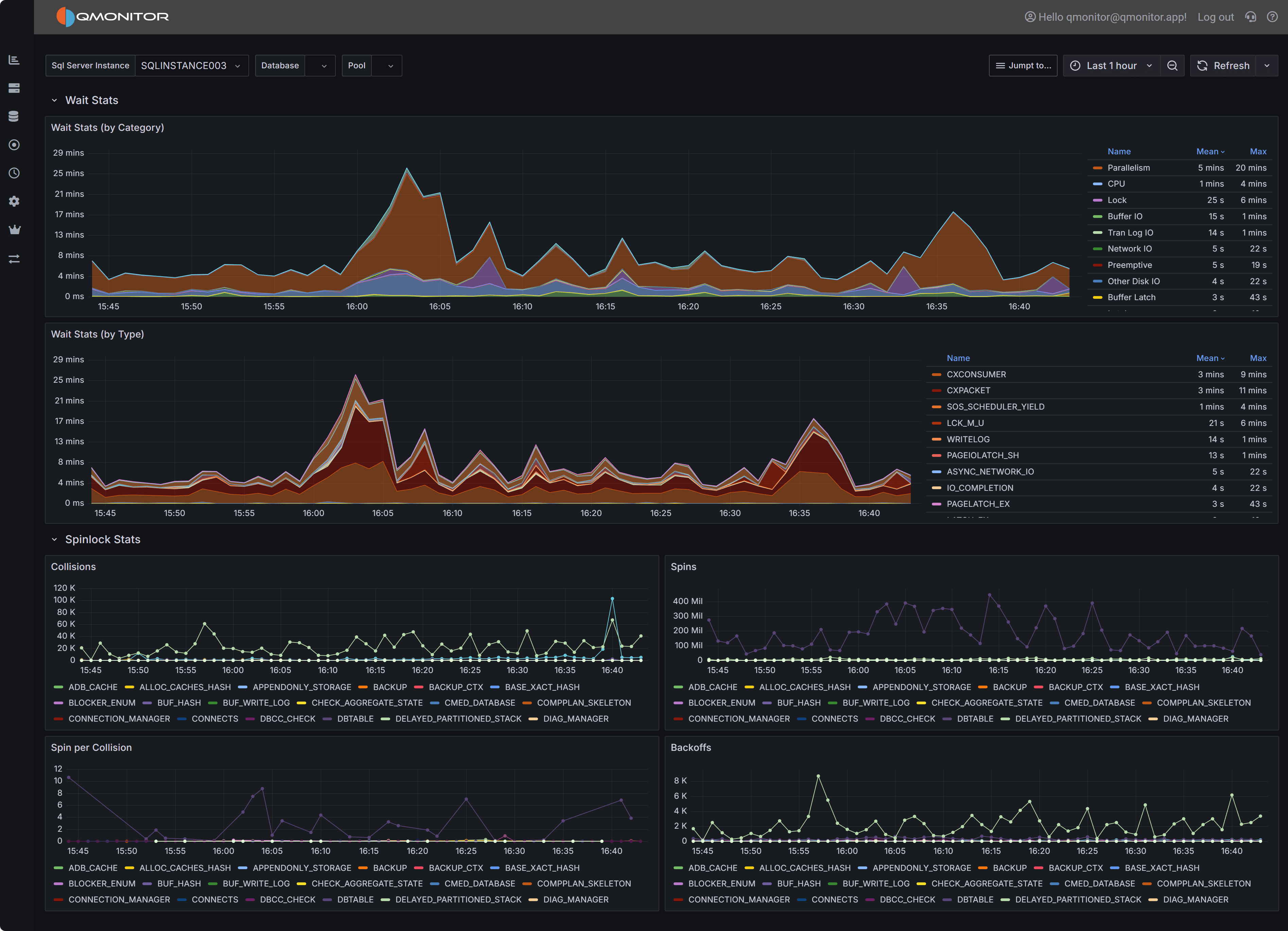Geek Stats dashboard showing wait statistics by category and type, plus spinlock metrics

Dashboard Sections

Wait Stats by Category

The Wait Stats by Category chart provides a high-level view of wait time grouped into categories such as I/O waits, CPU-related waits, lock/latch waits, network waits, and others. This stacked area chart shows how wait time is distributed across categories over the selected time interval.

This view uses the same wait categories as the Instance Overview dashboard, making it easy to drill down from high-level monitoring into detailed wait analysis. When the Instance Overview shows elevated wait times in a particular category, use this chart to see how that category’s wait time trends over a longer period and correlate spikes with specific time windows or workload patterns.

The chart legend on the right displays each wait category with its mean and maximum values during the selected interval. Common categories include:

• Replication: Waits related to database mirroring, Always On Availability Groups, or log shipping
• CPU: Waits indicating CPU pressure, such as SOS_SCHEDULER_YIELD
• Lock: Waits for locks on database objects
• Buffer IO: Waits for buffer pool I/O operations
• Tran Log IO: Waits for transaction log writes
• Network IO: Waits for network communication, such as ASYNC_NETWORK_IO
• Preemptive: Waits while SQL Server yields to external operations like extended procedures or CLR code
• Other Disk IO: Waits for disk operations not related to buffer pool or log
• Buffer Latch: Waits for latches on buffer pool pages

Use this chart to identify which broad wait category dominates during performance issues. For example, high Buffer IO and Tran Log IO categories suggest storage bottlenecks, while high CPU categories indicate scheduling pressure or insufficient CPU resources.

Wait Stats by Type

The Wait Stats by Type chart drills down to individual wait types, showing the exact SQL Server wait types contributing to performance issues. This stacked area chart displays specific wait types like PAGEIOLATCH_SH, CXPACKET, SOS_SCHEDULER_YIELD, ASYNC_NETWORK_IO, and many others.

Individual wait types provide precise diagnostic information about what SQL Server threads are waiting for:

CXCONSUMER and CXPACKET indicate parallel query coordination waits. High values may suggest inefficient parallelism, queries that would benefit from lower MAXDOP settings, or skewed data distribution causing uneven workload across parallel threads.

SOS_SCHEDULER_YIELD indicates threads yielding the CPU scheduler, often a sign of CPU pressure where more threads want CPU time than cores are available.

PAGEIOLATCH_ waits (SH, EX, UP) indicate threads waiting for data pages to be read from disk into the buffer pool. High values suggest memory pressure forcing excessive physical I/O, missing indexes causing table scans, or slow storage subsystems.

ASYNC_NETWORK_IO indicates SQL Server is waiting for the client application to consume result sets. This typically means the application is slow to process returned data, not a SQL Server performance issue.

IO_COMPLETION and related waits indicate threads waiting for disk I/O operations to complete, pointing to storage performance bottlenecks.

PAGELATCH_ waits indicate contention on in-memory page structures, often related to allocation contention (tempdb, table heaps) or hot pages with high concurrent access.

A complete list of wait types and their meanings is beyond the scope of this documentation, but comprehensive information can be found in Microsoft’s documentation for the DMV sys.dm_os_wait_stats.

The chart legend shows mean and maximum values for each wait type, helping you identify both consistent contributors and intermittent spikes. Sort or filter the legend to focus on top wait types.

Spinlock Stats

The Spinlock Stats section provides detailed metrics about spinlock activity within SQL Server. Spinlocks are lightweight synchronization primitives SQL Server uses to protect short-lived access to internal data structures. When multiple threads need simultaneous access to the same structure, spinlock contention occurs, causing threads to “spin” (busy-wait) and consume CPU while waiting.

Four charts visualize different aspects of spinlock behavior:

Collisions

The Collisions chart shows how often threads encountered contention when attempting to acquire spinlocks. Each collision represents a situation where a thread tried to acquire a spinlock but found it already held by another thread, forcing the thread to wait.

High collision counts indicate frequent contention on SQL Server’s internal structures. The chart displays collisions for specific spinlock types like SOS_CACHESTORE, LOCK_HASH, and others. Different spinlock types protect different internal structures, so identifying which types have high collisions helps pinpoint the source of contention.

Spins

The Spins chart displays the total number of spin attempts across all spinlock types. When a thread encounters a collision, it enters a spin-wait loop, repeatedly checking if the spinlock becomes available. The total spins metric shows the cumulative busy-wait activity.

High spin counts, especially when combined with high collisions, indicate threads are spending significant time in busy-wait loops rather than doing productive work. This wastes CPU cycles and can appear as high CPU utilization without corresponding application throughput.

Spins per Collision

The Spins per Collision chart shows the average number of spins required for each collision. This metric indicates how costly each contention event is: higher values mean threads spin longer before acquiring spinlocks.

Low spins-per-collision values (1-10) suggest brief contention quickly resolved. High values (100+) indicate spinlocks are held for longer periods, forcing waiting threads to spin extensively. This is particularly problematic because spinning consumes CPU without making progress.

Backoffs

The Backoffs chart shows how often threads backed off (yielded) after spinning. When a thread spins for a threshold number of iterations without acquiring the spinlock, SQL Server’s spinlock implementation causes the thread to back off: yield its CPU time and enter a wait state rather than continuing to spin.

High backoff counts indicate spinlock contention is severe enough that threads exhaust their spin attempts and must yield. This extends the time to acquire spinlocks and can lead to scheduling delays and reduced throughput.

Investigating Wait and Spinlock Issues

Correlating Waits with Performance Problems: When users report slow query performance, check the Wait Stats by Type chart during the problem time window. High PAGEIOLATCH waits suggest I/O bottlenecks:review the SQL Server I/O Analysis dashboard to confirm storage latency. High SOS_SCHEDULER_YIELD waits indicate CPU pressure: check CPU metrics in the Instance Overview dashboard. High lock waits suggest blocking: review the Blocking dashboard.

Identifying Query-Specific Wait Patterns: Use the Query Stats dashboard to identify expensive queries, then check their execution times against wait spikes in this dashboard. Queries with high wait times relative to CPU time are spending most execution time waiting rather than executing, indicating optimization opportunities.

Addressing High I/O Waits: PAGEIOLATCH and IO_COMPLETION waits indicate I/O bottlenecks. Investigate whether missing indexes are causing excessive table scans, whether memory pressure forces frequent physical reads, or whether storage performance is inadequate. Review buffer cache hit ratios and Page Life Expectancy in the Instance Overview dashboard. Consider adding memory, optimizing queries, or upgrading storage.

Resolving CPU-Related Waits: SOS_SCHEDULER_YIELD waits indicate CPU pressure from too many concurrent queries or CPU-intensive operations. Review the Query Stats dashboard to identify CPU-consuming queries. Consider adding CPU cores, optimizing expensive queries, or using Resource Governor to limit CPU consumption by specific workloads.

Diagnosing Spinlock Contention: High spinlock collisions and spins indicate contention on SQL Server’s internal structures. Common causes include:

• Tempdb allocation contention: Multiple sessions creating temporary objects simultaneously. Consider enabling tempdb metadata memory-optimized optimization (SQL Server 2019+) or adding more tempdb data files.

• Plan cache contention: Frequent plan compilation and eviction. Review whether forcing parameterization, increasing plan cache size, or using query hints would help.

• Lock hash contention: Many concurrent transactions acquiring locks. Consider partitioning hot tables, using read-committed snapshot isolation, or optimizing transaction patterns.

• Connection leakage: Applications that open many connections without properly closing them can cause excessive spinlock contention. Review application connection pooling and consider using connection pooling best practices.

Tracking Wait Trends Over Time: Use the time range selector to analyze wait patterns across different periods. Compare business hours versus off-peak times, weekdays versus weekends, or before/after application changes. Sudden changes in wait patterns often indicate workload shifts, application updates, or configuration changes that need investigation.

Related Dashboards

Use the Instance Overview dashboard for high-level wait category monitoring during routine operations. Drill into Geek Stats when you need detailed wait type analysis.

Review the Query Stats dashboard to identify which specific queries contribute to high waits. Understanding which queries wait and why guides optimization efforts.

Check the SQL Server I/O Analysis dashboard when I/O-related waits dominate to understand storage performance and identify bottlenecks.

Monitor the Capacity Planning dashboard alongside spinlock metrics. High spinlock contention combined with approaching CPU capacity limits may indicate you need more CPU cores or workload distribution.

Review the Blocking dashboard when lock waits are high to understand blocking chains and identify sessions holding locks that others need.

1.11 - Custom Metrics

This dashboard displays custom metric measurements pulled from the selected measurement source.

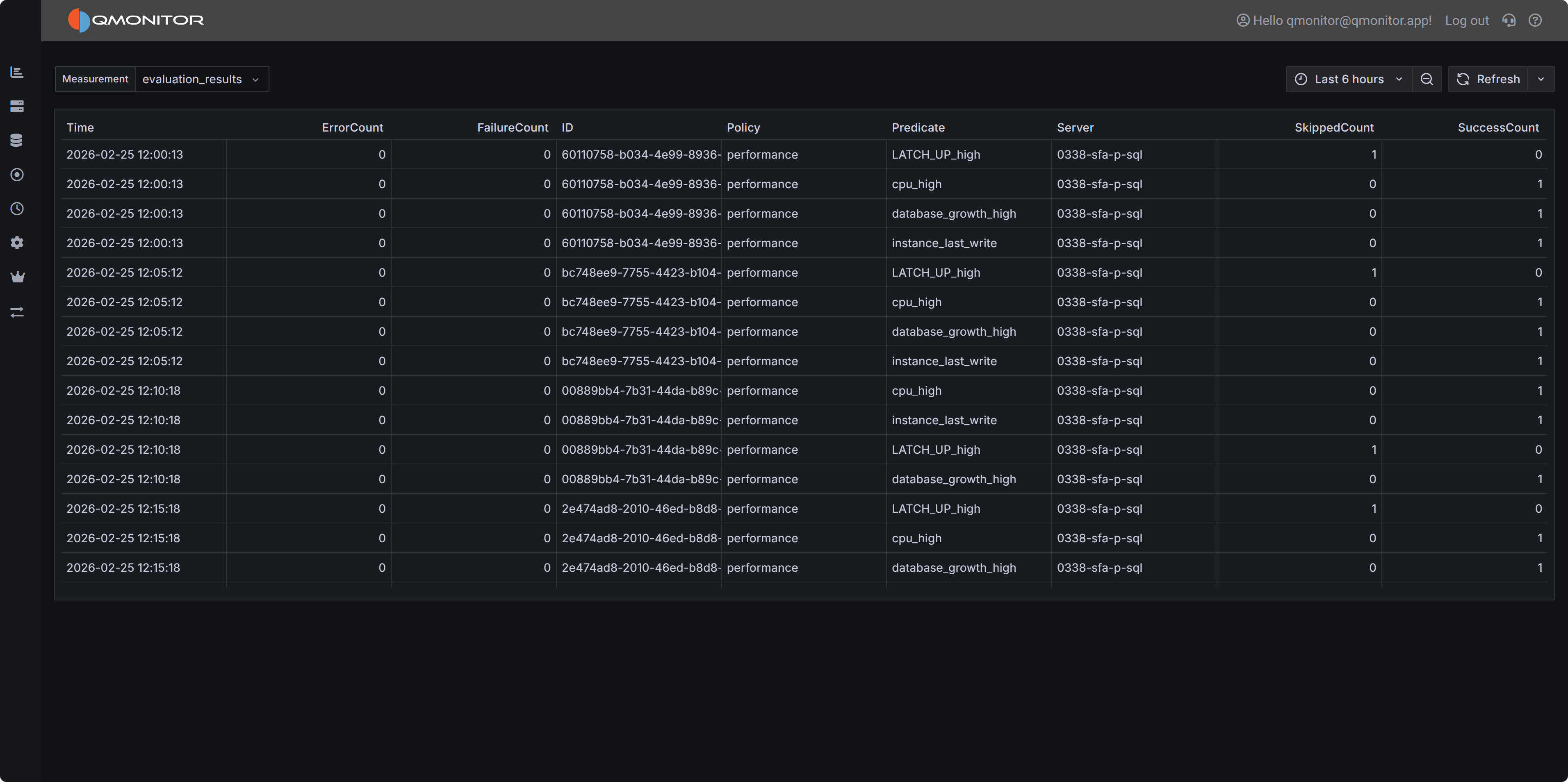Custom Metrics dashboard showing measurement data with time-series results

Top controls

• Measurement selector: a dropdown to choose which measurement to query.
• Time filter: applies the selected time window to the query.

Data table

• The table below the selector shows the measurement data for the chosen measurement and time range. Typical columns include timestamp, value, and any measurement tags or labels.
• The dashboard retrieves up to 10,000 data points for the selected query. If the time range or measurement produces more points, results are truncated to this limit.

Usage notes

• Select the desired measurement, choose an appropriate time window, and refresh the view to populate the table.
• Narrow the time range or apply server/instance filters when results are truncated due to the 10,000‑point limit.
• Export or copy table rows for offline analysis if needed.

Future capability

• We are working on support for creating custom dashboards directly from these measurements. This feature is in development and will be available soon.

2 - Issues

The Issues page lists all problems detected across your monitored SQL Server instances, helping you track configuration violations, performance issues, and operational concerns in one centralized view.

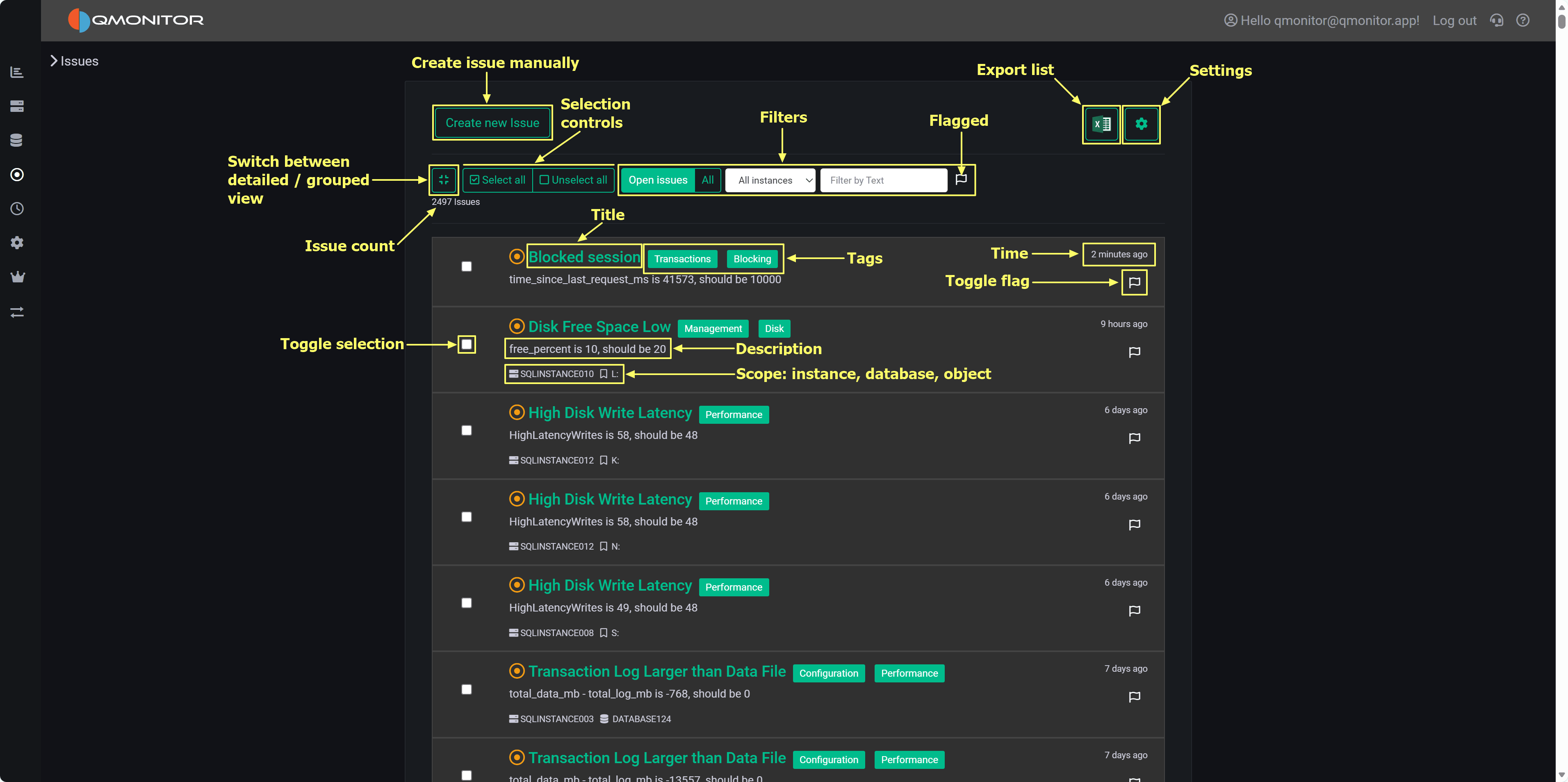Issues page showing detected problems with filtering and grouping options

How Issues Work

Issue Creation: Issues are automatically created when SQL Server instances violate rules defined in policies. Rules are organized as Policies (containers) and Predicates (individual checks). When a predicate fails evaluation, an issue is opened, similar to a ticket in an issue tracking system or a GitHub issue.

Evaluation Schedule: The background evaluation engine runs on a schedule:

• Diagnostic policy: Checks instance configuration and best practices once per day
• Performance policy: Evaluates runtime performance predicates every 5 minutes

Automatic Resolution: When a previously failing predicate passes in subsequent evaluations, the corresponding issue is automatically closed. The system prevents duplicate issues—if an issue already exists for a predicate/instance combination, it’s updated rather than creating a new issue.

Manual Issues: Use the Create new issue button to manually record problems not detected by policies, such as operational incidents, investigations, or tasks.

Page Controls

Top Toolbar

Left Side:

• View Toggle (grid icon): Switch between detailed view (individual issues) and grouped view (issues organized by predicate)
• Create new issue (green button): Manually create issues for ad-hoc tracking
• Select all / Unselect all: Bulk select issues for actions
• Close Selected: Appears when issues are selected; closes all selected issues in one operation

Center - Filters:

• Open issues / All: Toggle between open issues only (default) or include closed issues
• Instance dropdown: Filter by specific SQL Server instance
• Text search: Search issue titles, descriptions, or instance names
• Flagged only: Show only issues marked with the flag for follow-up

Right Side:

• Export (Excel icon): Download the current issues list as an Excel file
• Settings (gear icon): Open the Policies page to view and edit rules

Issue Count: Total number of issues matching current filters displays below the toolbar (e.g., “2496 Issues”)

Issue List Views

Detailed View (Default)

Each issue row displays:

• Checkbox: Select for bulk actions
• Title (green text): Predicate name describing the problem. Click to open the Issue Detail page with remediation guidance and evaluation history
• Description: Specific failing condition (e.g., “free_percent is 10, should be 20”)
• Category Tags: Colored badges (Performance, Management, Configuration, Disk, etc.) indicating issue type
• Scope: Instance name and affected object (database or component) shown with icons
• Created Date: Relative time when issue was opened (e.g., “2 minutes ago”, “6 days ago”)
• Flag Button (🚩): Click to mark/unmark the issue for follow-up

The list uses infinite scrolling to automatically load more issues as you scroll down.

Grouped View (By Predicate)

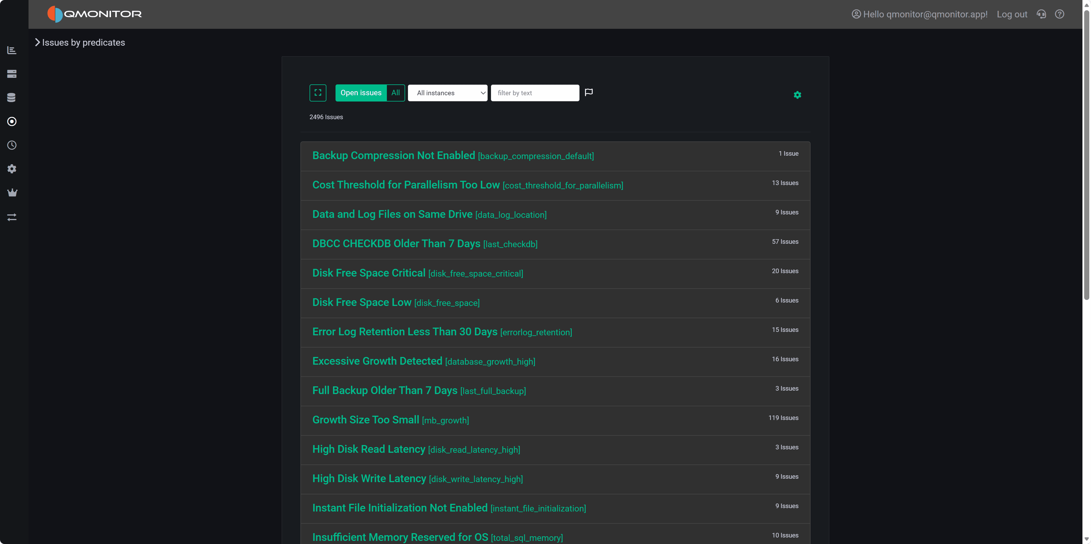Grouped view showing issue counts per predicate

Toggle to grouped view to see predicates with their issue counts instead of individual issues. Each row shows:

• Predicate name (green text) with internal identifier in brackets
• Issue count: Number of instances failing this predicate

Use grouped view to quickly identify frequently failing predicates and prioritize policy-level fixes. Click a grouped row to expand and see underlying issues or drill into the predicate detail page.

Working with Issues

Triaging: Start with Open + Flagged filter to focus on urgent problems. Flag critical issues using the flag button so they appear when this filter is active.

Bulk Operations: Select multiple issues using checkboxes, then click Close Selected to resolve them in one operation. This preserves issue metadata and records who closed them and when.

Filtering by Instance: Use the instance dropdown to focus on specific servers. This is particularly useful when different team members are responsible for different instances, or when investigating problems on a specific server.

Reviewing History: Switch to All (instead of Open issues) to include closed issues in the list. Review closed issues to analyze trends, understand recurring problems, or audit remediation efforts.

Exporting Data: Click the Excel icon to export the current filtered list. Use exports to share findings with stakeholders who don’t have QMonitor access, create reports for management, or perform offline analysis.

Viewing Details: Click any issue title to open the Issue Detail page showing:

• Complete problem description
• Suggested remediation steps
• Evaluation history showing when the issue was detected and resolved
• Related configuration or performance metrics

Managing Policies: Click the settings (gear) icon to open the Policies page where you can:

• View and edit policy configurations
• Adjust predicate parameters and thresholds
• Configure notification settings for specific rules
• Enable or disable predicates

Issue Categories

Category tags help you quickly identify issue types. Common categories include:

• Performance: Runtime performance problems (high latency, CPU pressure, memory issues)
• Configuration: Best practice violations or suboptimal settings
• Management: Operational concerns (backup issues, maintenance problems)
• Disk: Storage-related issues (low free space, slow I/O)
• Blocking: Query blocking and locking problems
• Transactions: Transaction log and commit issues

Best Practices

Daily Workflow: Check Open + Flagged issues each morning to identify overnight problems. Flag new critical issues as you review them so they’re easy to find later.

Documentation: When closing issues, document the resolution in the issue detail page. This creates a knowledge base for similar issues in the future.

Trend Analysis: Periodically review All issues (including closed) to identify recurring problems. Predicates that fail repeatedly may indicate underlying configuration issues, capacity constraints, or application patterns that need addressing at a higher level than individual issue resolution.

Policy Tuning: Use the grouped view to identify predicates generating excessive false positives. Adjust thresholds in the Policies page to reduce noise while maintaining protection for genuine problems.

2.1 - Issue Details

This page shows full context and actions for a single issue.

Top: Title and description

• Title: the issue title (often the predicate name for policy-generated issues).
• Description: a short statement of the failing condition. Example: “free_percent is 11, should be 20”.

Metadata

• Created: timestamp when the issue was opened.
• Instance: the SQL Server instance the issue refers to.
• Database / Object: the database or object name when applicable.

Explanation and remediation

• A concise explanation describes why the issue matters and recommended remediation steps. Include practical suggestions (for example: clear old files, adjust backup/retention policies, increase disk capacity, or change maintenance windows) and links to relevant documentation or runbooks.

Metric chart

• A time-series chart displays the metric evaluated by the predicate (for example, available disk space) over the selected interval. The chart shows values up to and including the point when the predicate was evaluated so you can see trend leading to the violation.

Policy evaluation details

• “Show Policy Evaluation Details” reveals the full evaluation record for the predicate: input properties, threshold values, measured value, evaluation timestamp, policy name, predicate id, and any additional diagnostic fields.
• Use this to verify the exact inputs that produced the issue.

Tags

• The Tags control lists tags assigned to the issue and lets you add or remove tags for workflow or routing (for example: “ops”, “storage”, “urgent”).

Closing notes

• Enter free-form notes describing how the issue was investigated or fixed.
• Notes are stored with the issue for audit and postmortem purposes.

Actions

• Save: persists tag changes and closing notes without changing issue state.
• Close issue: manually closes the issue. If the underlying predicate still fails on a subsequent automated evaluation, a new issue will be opened.
• Exclude: opens a dialog to disable this predicate for the specific instance/database/object/group/tag combination. The dialog also offers the option to close all matching issues for the selected scope. Use exclusions sparingly and document the rationale (ex. test instance).
• Fix issue: when available, this button schedules an automated remediation job that executes the predefined T-SQL script associated with the predicate. Not all issues support automatic fixes — availability depends on the predicate and the remediation defined for it. The jobs UI shows the script to be run, required permissions, and the scheduled job status. Execution logs and results are recorded with the job.

Behavior and history

• Closed issues remain available for historic review; use filters on the Issues list to include closed items.

2.2 - Policies

This page lists all Policies configured in the system.

Overview

• Each row shows a single Policy with its name and a short description.
• Click a Policy name to open the Predicates page, which lists every predicate (rule) contained in that Policy.

Enable / disable control

• A toggle beside each Policy enables or disables the Policy and all of its predicates in one action.
• Disabling a Policy prevents its predicates from being evaluated by the background engine and stops new issues from being created by those rules.
• Existing open issues created by predicates in a disabled Policy remain visible and can be closed manually; they are not automatically removed.

Usage notes

• Use the list to review which policy groups are active (for example, Diagnostic vs Performance) and to temporarily suspend evaluation during maintenance windows or policy tuning.
• Click through to Predicates to adjust individual rules, or thresholds.

2.3 - Predicates

This page lists all predicates defined for the selected Policy.

Predicates list

• Each row represents a single predicate with concise metadata:
  • Name: predicate identifier (click to open predicate detail).
  • Enabled: toggle to enable or disable the predicate evaluation.
  • Notify: toggle to enable or disable notifications for this predicate.

Behavior

• Disabling a predicate prevents the evaluation engine from running that predicate and stops new issues from being created by it.
• Disabling notifications suppresses alerting for failures; issues are still created and tracked, but no notifications are sent for those events.

Controls and actions

• Click the predicate name to go to the predicate details page
• Use the inline toggles to quickly enable/disable predicates or notifications.

Usage tips

• Use the Notifications toggle to mute noisy predicates while retaining the audit trail of issues.
• Disable a predicate only when you are certain the check is irrelevant or will cause false positives; prefer tuning thresholds where possible.

Overrides and defaults

• Predicates use shared default values for thresholds, enabled state, and other properties. All organizations inherit the same defaults but may override them as needed.
• Overrides can be applied at two scopes:
  • Global: applies everywhere the predicate is used.
  • Scoped: applies to a specific combination of instance, database, object, group, or tag. For example, an override on a tag affects all instances that have that tag; an override on a specific SQL instance affects only that instance.
• Changing any predicate property (including disabling it) counts as an override because the predicate’s effective configuration differs from the shared default.
• Predicates that have overrides are shown beneath the original unmodified predicate. Overrides are highlighted (orange text) to distinguish them from the default predicate rows (green).
• When an override is scoped to instance/database/object/group/tag, the override row displays the scope information so you can see exactly where the change applies.
• To remove an override and revert to the default behavior, use the delete icon on the right of the override row. Deleting the override restores the predicate to the shared default values.

Exclude from evaluation via an issue

• The “Exclude” action available on an Issue creates the same kind of override described above. When you open the Exclude dialog from an Issue you are setting the predicate’s enabled state to off for the scope you select.
• The dialog presents checkboxes for scope selection: instance, database, object, group, and tag. Selecting one or more scopes creates a scoped override (enabled = off) that prevents the predicate from running for that specific combination.
• Excluding from an Issue can optionally close all matching open issues for the selected scope; the override itself is recorded and shown under the predicate (highlighted in orange).
• Exclusions are reversible: delete the override row to restore the default behavior, or edit the override to change its scope or enabled state.

2.4 - Predicate Details

This page contains a form to view and edit all properties of a predicate, including scoped overrides and the evaluation expressions used by the background engine.

Scope controls

• Server Tag: apply this predicate only to servers that have the selected tag.
• Server Group: limit the predicate to servers belonging to a specific group.
• Server: target a single SQL instance for this override.
• Database: restrict the predicate to a particular database.
• Object: restrict the predicate to a specific object (for example, a file, table, or index).
• Use the scope controls to create a scoped override; leaving a field empty makes the override less specific (broader).

Editable expressions and fields

• Evaluation Expression: the boolean expression the engine evaluates. The default is “actual = expected”, but you can change this to any valid expression supported by the engine (for example “actual < expected” or “actual > low AND actual < high”).
• Expected Expression: the expected value or expression to compare against. This may be a constant (e.g., 20), a computed expression, or one of the available properties of the object being checked.
• Actual Expression: the expression that yields the measured value to be evaluated (typically the name of a property from the underlying object, e.g., free_percent or file_size_gb).
• Property Name: the logical name used to identify the property in UIs and reports. It maps the actual expression to a friendly identifier and can be used by other parts of the system to reference this value (for example in charts or exported data).
• Filter Expression: an optional expression that narrows the set of objects the predicate applies to. Use it to include or exclude specific objects so the check only runs against matching items (for example: database_name = ‘X’ AND file_type = ’log’).

Behavior and helpers

• Save applies the changes and creates or updates an override for the selected scope. Changing any property (including disabling) counts as an override.

3 - Settings

The Settings page lets you configure personal preferences and organization defaults that affect how QMonitor behaves for your user and the orgs you manage.

Account management

• Manage your account: button at the top of the page that opens your Account page. Use the Account page to update your email, password, 2FA, and personal contact details.

Appearance

• Theme: choose Light or Dark theme for the application. The selected theme is applied immediately after you click Save.
• Time zone: select the time zone used to display timestamps in the UI for your user. Note: the time zone setting applies only to your user profile, not to the organization or other users.
• Save applies appearance changes and persists them to your profile.

Organizations

• Current organization: the name of the organization you are currently scoped to is shown near the top of the organizations section.
• Manage organization: button opens the Manage Organization page where you can change org-level settings, members, and billing (if permitted by your role).
• Organization actions:
  • Join organization: request to join an existing organization.
  • Create new organization: start a new organization and become its owner.
  • Switch organization: change your active organization context when you belong to multiple organizations.

Behavior and tips

• Personal settings (theme and time zone) are stored per user and follow you across devices when you sign in.
• Organization management actions depend on your role and permissions; some controls may be hidden if you lack admin privileges.
• Use Save to persist changes; unsaved edits are not applied to your session.

Accessibility and support

• Changing theme can improve readability and reduce eye strain for long sessions; use the Dark theme for low-light environments.
• If you need assistance managing account or organization settings, contact your org administrator.

3.1 - Preferences

3.2 - Manage Organization

The Manage Organization page is where organization owners configure org-level settings, membership, billing, and branding. Access to this page is restricted to organization owners and administrators; non-admin users can view fewer options or receive an access denied message.

Left-hand tabs

• General: edit the organization name and display name
• Notifications: configure global notification channels
• Billing Details: enter or update billing contact, billing address, and tax information used on invoices.
• Licenses: view current license counts and usage, purchase additional seats, or renew expiring licenses.
• Payment History: review past invoices, payments, and subscription activity.
• Members: invite, remove, or change roles for organization members; manage pending invitations and role-based permissions.
• Customize: upload organization logo and set branding options shown in the UI and on shared reports.

3.2.1 - General Options

Organization name and display name

• Display Name: a human-friendly name shown in the UI and reports.
• Actual Name: a machine-safe identifier used by tooling (ConfigWizard, ConfigWizardCmd, agents). The actual name is sanitized to remove or replace characters that could break scripts or client tools; avoid spaces and punctuation when choosing an organization name.

Default instance settings

• “Acknowledge you are running jobs as a sysadmin”: when checked, new instances registered in this organization will have the same acknowledgement enabled by default. This setting simply controls the default for newly added instances and can be changed per-instance later.

Organization key

• Regenerate organization key: use this to replace the org key if it is lost or compromised. Regenerating the key immediately invalidates the current key — all existing agents and integrations using the old key will stop communicating and must be reconfigured with the new key. Confirm this action only after planning for agent reconfiguration.

Delete Organization

• Delete organization: permanently removes the Organization and all org- scoped data. This action is irreversible and requires explicit confirmation (type-to-confirm). Only organization owners can perform deletion.

3.2.2 - Notifications

This page configures how your organization receives alerts from QMonitor. Use these settings to deliver operational notifications to the right channels and reduce noise by choosing appropriate delivery methods per severity.

From the Notification settings page you can enable one or more channels and test each configuration before saving.

Supported notification channels

QMonitor currently supports the following notification channels:

• Email
• Microsoft Teams
• Telegram
• Slack

Each channel can be enabled independently and tested using the Test button available next to the configuration fields.

Email notifications

1. Enable Email
2. Enter one or more email addresses (use commas to separate multiple recipients)
3. Click Test to verify delivery
4. Save the configuration

Microsoft Teams notifications

QMonitor sends notifications to Microsoft Teams using an Incoming Webhook URL. Messages are delivered to a specific channel as Adaptive Cards and may include text and images (graphs associated with issues).

How to enable

1. In Microsoft Teams, open the target Team and Channel
2. Click More options next to the channel name
3. Select Workflows
4. Create a new Incoming Webhook
5. Copy the generated Webhook URL
6. Paste it into QMonitor → Teams webhook url
7. Click Test to verify delivery
8. Save the configuration

If you do not have access to the Workflows section contact your Teams administrator

Telegram notifications

Telegram notifications are sent by a Telegram bot to a channel.

Step-by-step setup

1. Create the bot

1. Open Telegram and search for @BotFather
2. Send:

   /newbot
   

3. Choose a name and a username

BotFather will return a Bot Token like:

123456:ABC-defGHI...

This value goes into Bot token in QMonitor.

2. Create a Telegram channel

1. Telegram → New Channel
2. Choose a name
3. Set it as Private (recommended)
4. Create the channel

3. Add the bot as administrator

1. Open the channel → Info → Administrators
2. Add your bot (e.g. @thenameyouchooseearlier)
3. (Mandatory) Grant at least “Can post messages” permission

4. Retrieve the Channel Chat ID

1. Send any message in the channel
2. Open in a browser:

   https://api.telegram.org/bot<YOUR_BOT_TOKEN>/getUpdates
   

3. Look for the chat section in the JSON response:

"chat": {
  "id": -1003314549127,
  "title": "ChannelName",
  "type": "channel"
}

The Chat ID is the negative number (e.g. -1003314549127).

Final parameters to enter in QMonitor

• Bot token → Telegram bot token
• Chat ID → Channel chat ID

After saving, use Test to confirm delivery.

Slack notifications

Slack notifications support:

• Text messages via Incoming Webhooks
• Images (optional) via Slack Bot API

1. Create a Slack App

1. Go to https://api.slack.com/apps
2. Click Create New App → From scratch
3. Choose a name (e.g. QMonitor)
4. Select the workspace

2. Enable Incoming Webhooks (required)

1. Features → Incoming Webhooks
2. Activate Incoming Webhooks → ON
3. Add New Webhook to Workspace
4. Select the target channel
5. Copy the Webhook URL

This value goes into Slack Incoming Webhook URL.

3. Enable image upload (optional)

Required only if you want to also see the notification’s associated images (graphs contained in issues).

Add the following bot scopes in OAuth & Permissions:

• chat:write
• files:write
• channels:read
• groups:read (only for private channels)

After adding scopes, reinstall the app.

4. Retrieve Bot Token

Copy the Bot User OAuth Token (xoxb-…).

This value goes into Slack Bot token.

5. Retrieve Channel ID

Open Slack in the browser and navigate to the channel.

URL example:

https://app.slack.com/client/TXXXXXXX/CYYYYYYY

Use CYYYYYYY (public) or GYYYYYYY (private).

This value goes into Slack Channel ID.

6. Invite the bot to the channel

Inside the Slack channel, run:

/invite @QMonitor

Without this step, image uploads will not be visible.

Final parameters to enter in QMonitor

• Webhook URL → required
• Bot token → required only for images
• Channel ID → required only for images

Use Test to confirm correct delivery.

3.2.3 - Billing Details

Billing information form

• The Billing info section is a form where you enter your company’s billing details used to generate invoices. Typical fields include company name, billing address, VAT number / fiscal code, contact name, email, and phone.
• Changing the country in the form will show or hide additional country- specific fields. For example, selecting Italy exposes “Certified Email Address (PEC)” and “SDI Code” fields required on Italian invoices.
• The information you provide here is printed on invoices. Keep it accurate to avoid delays or invoice re-issues.

Purchase prerequisites and VAT rules

• You must complete the billing form before purchasing licenses; the system will block checkout until required billing fields are provided.
• EU reverse-charge VAT: if your company is in an EU country, reverse-charge treatment applies only when you supply the required identifiers (for example VAT Number and/or national fiscal code as applicable). If you do not provide the necessary information, VAT will be applied to the license price and included on the invoice.

Sanctions and restricted sales

• We cannot sell licenses to entities or individuals located in countries sanctioned by the European Union or the Italian Republic. This includes, but is not limited to, Russia, Iran, and Afghanistan.
• If your billing address or company registration is in a sanctioned jurisdiction, purchases will be declined.

Tips and support

• Use official company identifiers (VAT or fiscal codes) to ensure correct tax treatment and avoid invoice corrections.
• If you need assistance completing country-specific fields, contact your finance team or open a support ticket via the Help menu.

3.2.4 - Licenses

The Licenses page lists all available licenses and provides actions to renew or manage them.

License list

• Columns shown for each license:
  • Valid to: the license expiry date.
  • Name: a friendly name or a GUID that identifies the license.
  • Assigned to: the SQL instance the license is assigned to; blank if not assigned.
• Each row has a checkbox so you can select one or more licenses for bulk actions.

Renewal and payment

• Use the “Renew # licenses” button to proceed to the payment page and renew the selected licenses.
• Payment is processed by Stripe; QMonitor does not store payment methods or credit card numbers.

Actions and notes

• Select multiple rows to renew licenses in bulk.
• Assigned/unassigned status is shown in the table; use the button at the top of the list to assign licenses

Assign vacant licenses

• When you have multiple licenses available, use the “Assign licenses” button to automatically allocate vacant licenses to instances that do not currently have a license. The assignment process selects unassigned licenses and binds them to unlicensed instances until either all selected licenses are used or all instances are licensed.

3.2.5 - Payment History

The Payment History page lists all payments and invoices for the organization. Use this view to review past charges, download invoices, and reconcile billing.

Payments table

• Columns:
  • Date: payment or invoice date.
  • Paid: amount actually paid (currency).
  • Total: invoice total before/after taxes as shown on the invoice.
  • Invoice: link to the invoice document (PDF).

Actions and filters

• Click an Invoice link to download or open the invoice PDF for accounting.

Notes

• Payment method and transaction details are recorded with each entry.
• For billing questions or disputes, contact billing support

3.2.6 - Members

This page lets organization owners manage access and invitations.

Access and invitations

• Initially only organization owners can access the Manage Organization pages.
• Owners can invite new users with the “Invite” button at the top-right.
• The invite dialog lets you enter an email address or copy an invitation code to share directly. The dialog shows the code immediately for manual distribution.
• The invited user receives an email with the invitation link and code. If the user is not registered, they must sign up first and then redeem the invitation code or follow the link to join the organization.

Members list

• The members table shows current organization users with simple controls:
  • Email: the member’s email address.
  • Role: a dropdown to change the member role (Owner or User).
  • Delete: remove the member from the organization.
• Role changes and removals may require confirmation.

Behavior and tips

• Use Owner role sparingly; owners can manage billing, policies, and members.
• Prefer inviting users to a role of “User” and elevate to Owner only when necessary.
• Invitations expire after a limited time; resend if a user reports an expired invite.

3.2.7 - Logo and Branding

Organization logo

• Current logo: the page displays the organization’s current logo for both themes so you can verify what users see.
• Theme-specific logos: you can upload a separate logo for Light and Dark themes to ensure good contrast and legibility in both modes.
• Upload controls: choose a file for the Light logo and a file for the Dark logo. Supported formats: PNG and SVG. Recommended dimensions: provide a high-resolution square or horizontal asset; SVGs scale crisply for all sizes.

Preview and reset

• Preview: the preview area shows how the selected logos and accent color will appear in the UI before you save changes.
• Reset: click Reset to revert the logo for the current theme back to the product default. Reset does not affect the other theme’s logo unless you reset it as well.

4 - Jobs

This page lists scheduled jobs and provides controls to create, filter, inspect, and clean up job records.

Top controls

• Create new job: opens the New Job page to define a job and its schedule.
• Filters:
  • Job status: All, Not run, Failed, Succeeded, Executed — use this to focus on the executions you care about.
  • Instance: restrict the list to a single SQL instance.
  • Job type: Manual jobs or Autofix jobs (automatic remediation).
• Delete completed one-time jobs: removes completed jobs that had a one-time schedule to tidy the list and reclaim storage.

Jobs list

• The list shows jobs matching the selected filters. Each row contains:
  • Job status icon: visual state of the latest execution
    • Green checkmark = completed successfully
    • Blue spinner = running/in progress
    • Red X = failed/error
  • Job type: indicates the action (Execute query or Execute command).
  • Name: job name; next to it (in smaller text) the schedule description (for example “at 02:00” or “On 2025-11-01 at 09:00”).
  • Delete: button to remove the job definition and its history.
  • Show log: opens the execution log for the job to inspect output, errors, and step details.

Row actions and navigation

• Click the job name to open the Job Detail page to edit or view the job.
• Use Show log to view recent runs, stderr/stdout, and execution status.
• Use Delete to remove obsolete jobs.

Tips

• Filter by Failed to quickly find jobs that need attention.
• Use the Instance filter to hand off job issues to the responsible DBA.
• Regularly remove one-time completed jobs to keep the job list manageable.

4.1 - Job Detail

This page lets you review, create, and edit a scheduled job and its settings. Jobs can execute a T-SQL query against one or more instances or run an arbitrary command on one or more agents.

Job properties

• Name: descriptive job name.
• Type: choose the job type:
  • Execute Query — runs the specified SQL text against selected SQL instances.
  • Execute Command — runs the specified command on one or more agents.

Execute Query controls

• Instance selection:
  • First dropdown: choose selection mode (Instance, Instance Group, or Tag).
  • Second dropdown: pick one Instance, Group, or Tag depending on the selection mode. Use groups or tags to target many instances.
• Max Concurrent Instances: maximum parallel executions:
  • 1 = run sequentially (no parallelism).
  • 0 = run against all selected instances in parallel.
  • Choose a limit to avoid saturating CPU, I/O, or network (for example, limit concurrent backups to 5 to avoid disk flooding).
• Retries: number of retry attempts on failure.
• Retry delay (s): delay, in seconds, between retry attempts.

Execute Command controls

• Agent target: choose All Agents or select a specific agent to run the command. Commands are executed by the agent process on the host running the selected agent(s).

Common controls (both job types)

• Enabled: checkbox that enables or disables the job without deleting it.
• Command: text area containing the T-SQL script or shell command to execute.
  • For Execute Query jobs, SQL text runs against the target instances.
  • For Execute Command jobs, the text is executed by the agent on the host.
• Schedule: click “Edit Schedule” to expand schedule settings:
  • Type: Recurring or One-time.
  • Cron Expression: enter a cron expression to define recurring schedules.
    • Help: the Help button opens documentation that assists in crafting valid cron expressions.
  • End Date: optional date when the schedule stops running.

Actions (bottom toolbar)

• Save: persist job definition and schedule.
• Run Now: immediately queue the job for execution (bypasses the schedule).
• Job Logs: open the job logs page to inspect past runs and execution output.
• Cancel: discard unsaved changes and return to the Jobs list.

Notes and tips

• Use small, targeted schedules during testing and run “Run Now” to validate behavior before enabling wide production schedules.
• Restrict Max Concurrent Instances for heavy operations (backups, restores, large ETL) to prevent resource contention.
• Commands executed by agents require appropriate agent permissions on the host
• Sysadmin acknowledgement
  • If an agent connects to a SQL instance using sysadmin credentials, the job will only run if the instance definition includes the “Acknowledge you are running jobs as a sysadmin” checkbox. This guard prevents accidental execution of high-privilege operations on instances where explicit consent has not been given.
  • Toggle the acknowledgement on the Instance Details page. Jobs that require sysadmin rights will display a warning if the acknowledgement is not enabled for the target instance.

4.2 - Job History

The Job History page displays past executions of scheduled jobs and their status so you can inspect runs, troubleshoot failures, and audit activity.

History table

• Columns:
  • Date and time: when the execution started (or completed).
  • Status: running, succeeded, or error (iconized for quick scanning).
  • Agent name: the agent that performed the execution.
• The list is ordered by date (newest first) and supports infinite scroll

Row details

• Click a row to expand detailed execution information:
  • A chronological list of log entries and messages produced during the run.
  • Standard output and standard error snippets (when available).
  • Execution duration, exit code, and retry attempts.
• Use expanded details to diagnose failures, identify error messages, and locate the exact step that failed.